Do you want BuboFlash to help you learning these things? Or do you want to add or correct something? Click here to log in or create user.
Subject 6. Profit Maximization
#cfa #cfa-level #economics #has-images #microeconomics #reading-15-demand-and-supply-analysis-the-firm
The goal of each firm is to maximize economic profit, which equals total revenue minus total cost.
- Total cost is the opportunity cost of production, which includes normal profit.
- Under perfect competition, a firm's total revenue equals price, P, multiplied by quantity sold, Q, or P x Q.
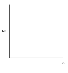
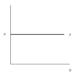
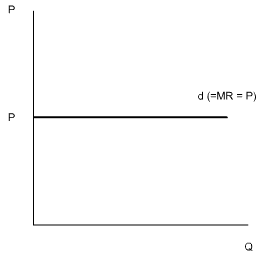
Marginal revenue is the addition to total revenue earned by a firm when one more unit of output is sold: MR = ΔTR/ΔQ. Since each unit of output sold by a price taker is sold at the market price, the MR for each unit is also equal to the market price, i.e., P = MR.
MR plotted against quantity sold would thus yield the same curve as P plotted against quantity sold (i.e., the demand curve) for the price taker.


We say that the MR curve of a price taker lies on the demand curve of a price taker.

There are three approaches to calculating the point of profit maximization in the short run. All three approaches yield the same profit-maximizing quantity of output.
MC = MR Approach
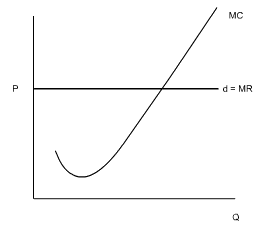
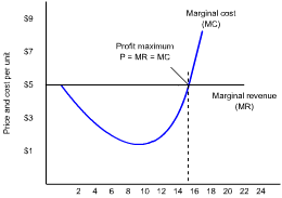
Produce that quantity of output where: MC = P = MR
- Each unit of output produced and sold by a price taker will generate revenue that equals the market price of the product (MR).
- However, due to the law of diminishing returns, as output increases, costs per unit will eventually also begin to increase (MC).
- The profit-maximizing quantity of output occurs where MC = MR = P.
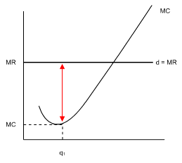
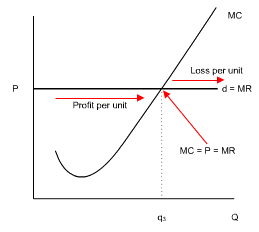
Here are two familiar curves: the MC curve and the MR curve of a certain firm. Note that the MC curve clearly illustrates the Law of Diminishing Returns. Given this information, what quantity of output should this profit-maximizing price taker produce?

What about producing q1 units?

Can you see that at q1, MR exceeds MC by the distance shown by the arrow? This means that the revenue received from the sale of that unit would exceed the cost of its production, so it would be profitable for the firm to produce that unit. But would the firm be maximizing its profits, or should the firm produce more?
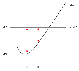
What about producing q2 units?

MR still exceeds MC, shown by the distance of the arrow. This means that the revenue received from the sale of unit q2 also exceeds its cost of production, so the firm would make even more profit if it produced that unit too.
But would the firm be maximizing its profits? Could the firm produce still more units?
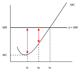
At q3, the MR earned from the sale of the unit is equal to the MC involved in producing the unit, so unit q3 generates neither a profit nor a loss for the firm.

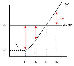
If the firm produced more than q3 units, the associated MC per unit would exceed the MR and each unit would incur a loss for the firm.

q4 incurs a loss since MC exceeds MR shown by the distance of the red arrow marked "Loss."
Hence, in the short run, the price taker will expand output until MR (the price charged) is just equal to MC. This enables the price taker to maximize its profits (or minimize its losses).

TR - TC Approach
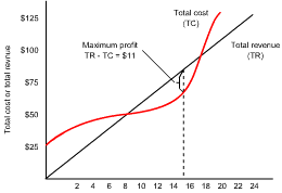
The rule is: find that quantity of output where TR exceeds TC by the most.


This is an alternative to the previous approach. The maximum distance between the total revenue (TR) and total cost (TC) curves of the firm will indicate where TR exceeds TC by the most - the quantity to be produced to maximize profits.
Input Approach
A third approach compares the revenue generated by each resource unit with the cost of that unit. Profit contribution occurs when the revenue from an input unit exceeds its cost. The point of profit maximization is reached when resource units no longer contribute to profit.
Profit Maximization in the Long Run
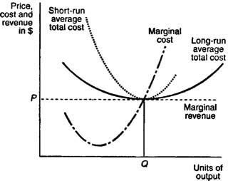
In the long run, firms can vary all of their input factors. A perfectly competitive firm can adjust the amount it uses of all factor inputs, including those that are fixed in the short run. For example, in the long run, the firm can adjust the size of its factory. In making these adjustments, the firm will seek to minimize its long-run average total cost. If, in the short run, the firm is operating below its minimum efficient scale and experiencing economies of scale, in the long run it can adjust its use of factor inputs so as to increase its output to the minimum efficient scale level.

The profit-maximizing level of output, where marginal cost equals marginal revenue, results in an equilibrium quantity of Q units of output. Because the firm's average total costs per unit equal the firm's marginal revenue per unit, the firm is earning zero economic profits. Furthermore, the firm is shown to be producing at the minimum point of its long-run average total cost curve, at the minimum efficient scale level of output.
The Long-Run Industry Supply Curve
The short-run market supply curve is just the horizontal summation of all the individual firm's supply curves. The long-run market supply curve is found by examining the responsiveness of short-run market supply to a change in market demand.
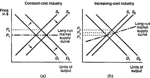
Consider the market demand and supply curves depicted in figures (a) and (b). Here, the market demand curves are labeled D1, and D2, while the short-run market supply curves are labeled S1 and S2.

Figure (a) depicts demand and supply curves for a market or industry in which firms face constant costs of production as output increases. At the intersection of D1 and S1, the market is in long-run equilibrium at a market price of P1. An increase in demand from D1 to D2 results in a new, higher market price of P2. In the short run, existing firms in this market will earn positive economic profits. In the long run, however, new firms will enter, causing short-run market supply to shift from S1 to S2 and driving the market price back down to P1. The long-run market supply curve is therefore given by the horizontal line at the market price, P1.
Figure (b) depicts demand and supply curves for a market or industry in which firms face increasing costs of production as output increases. Starting from a market price of P1, an increase in demand from D1 to D2 increases the market price to P2. In the short run, firms are earning positive economic profits. In the long run, new firms will enter the market, the short-run supply curve will shift from S1 to S2, and the new market price will be P3. The new, long-run market price of P3 is greater than the old market price of P1 because in an increasing-cost industry, the firm's average total costs rise as it produces more output. Thus, the long-run market supply curve in an increasing-cost industry will be positively sloped.
The path taken by an industry depends on underlying changes in resource prices and production cost. If expansion causes lower resource prices and production cost, then the result is a decreasing-cost industry. In this case, the long-run supply curve will be negatively sloped.
If you want to change selection, open original toplevel document below and click on "Move attachment"
Summary
| status | not read | reprioritisations | ||
|---|---|---|---|---|
| last reprioritisation on | suggested re-reading day | |||
| started reading on | finished reading on |
Details
Discussion
Do you want to join discussion? Click here to log in or create user.