on 14-Apr-2022 (Thu)

No interference means that my outcome is unaffected by anyone else’s treatment. Rather, my outcome is only a function of my own treatment. We’ve been using this assumption implicitly throughout this chapter. We’ll now formalize it. Assumption 2.4 (No Interference) 𝑌 𝑖 (𝑡 1 , . . . , 𝑡 𝑖−1 , 𝑡 𝑖 , 𝑡 𝑖+1 , . . . , 𝑡 𝑛 ) = 𝑌 𝑖 (𝑡 𝑖 ) Of course, this assumption could be violated. For example, if the treatment is “get a dog” and the outcome is my happiness, it could easily be that my happiness is influenced by whether or not my friends get dogs because we could end up hanging out more to have our dogs play together

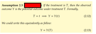
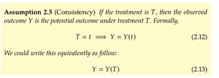
Consistency is the assumption that the outcome we observe 𝑌 is actually the potential outcome under the observed treatment 𝑇

It might seem like consistency is obviously true, but that is not always the case. For example, if the treatment specification is simply “get a dog” or “don’t get a dog,” this can be too coarse to yield consistency. It might be that if I were to get a puppy, I would observe 𝑌 = 1 (happiness) because I needed an energetic friend, but if I were to get an old, low-energy dog, I would observe 𝑌 = 0 (unhappiness). However, both of these treatments fall under the category of “get a dog,” so both correspond to 𝑇 = 1 . This means that 𝑌(1) is not well defined, since it will be 1 or 0, depending on something that is not captured by the treatment specification. In this sense, consistency encompasses the assumption that is sometimes referred to as “no multiple versions of treatment.”

stable unit-treatment value assumption (SUTVA)

SUTVA is satisfied if unit (individual) 𝑖 ’s outcome is simply a function of unit 𝑖 ’s treatment. Therefore, SUTVA is a combination of consistency and no interference (and also deterministic potential outcomes)

Assumptions of causal inference:

1. Unconfoundedness (Assumption 2.2)

2. Positivity (Assumption 2.3)

3. No interference (Assumption 2.4)

4. Consistency (Assumption 2.5)

An estimate (noun) is an approximation of some estimand, which we get using data

An estimand is the quantity that we want to estimate.

When we say “identification” in this book, we are referring to the process of moving from a causal estimand to an equivalent statistical estimand

When we say “estimation,” we are referring to the process of moving from a statistical estimand to an estimate

What do we do when we go to actually estimate quantities such as 𝔼 𝑋 [ 𝔼[𝑌 | 𝑇 = 1, 𝑋] − 𝔼[𝑌 | 𝑇 = 0, 𝑋] ] ? We will often use a model (e.g. linear regression or some more fancy predictor from machine learning) in place of the conditional expectations 𝔼[𝑌 | 𝑇 = 𝑡, 𝑋 = 𝑥] . We will refer to estimators that use models like this as model-assisted estimators. Now that we’ve gotten some of this terminology out of the way, we can proceed to an example of estimating the ATE

A graph is a collection of nodes (also called “vertices”) and edges that connect the nodes.

If there is a directed path that starts at node 𝑋 and ends at node 𝑌 , then 𝑋 is an ancestor of 𝑌 , and 𝑌 is a descendant of 𝑋

We will denote descendants of 𝑋 by de(𝑋)

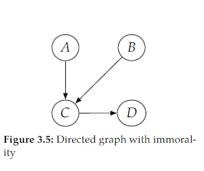
If two parents 𝑋 and 𝑌 share some child 𝑍 , but there is no edge connecting 𝑋 and 𝑌 , then 𝑋 → 𝑍 ← 𝑌 is known as an immorality

For example, if we remove the 𝐴 → 𝐵 to get Figure 3.5, then 𝐴 → 𝐶 ← 𝐵 is an immorality

It turns out that much of the work for causal graphical models was done in the field of probabilistic graphical models. Probabilistic graphical models are statistical models while causal graphical models are causal models.

Probabilistic graphical models are statistical models while causal graphical models are causal models.

Assumption 3.1 (Local Markov Assumption)

Given its parents in the DAG, a node 𝑋 is independent of all its non-descendants

The Bayesian network factorization is also known as the chain rule for Bayesian networks or Markov compatibility.

As important as the local Markov assumption is, it only gives us information about the independencies in 𝑃 that a DAG implies. It does not even tell us that if 𝑋 and 𝑌 are adjacent in the DAG, then 𝑋 and 𝑌 are dependent. And this additional information is very commonly assumed in causal DAGs. To get this guaranteed dependence between adjacent nodes, we will generally assume a slightly stronger assumption than the local Markov assumption: minimality

Assumption 3.2 (Minimality Assumption)

1. Given its parents in the DAG, a node 𝑋 is independent of all its non-descendants (Assumption 3.1).

2. Adjacent nodes in the DAG are dependent.

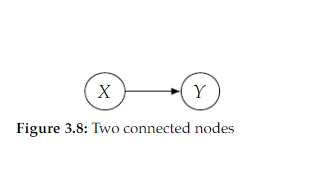
For example, if the DAG were simply two connected nodes 𝑋 and 𝑌 as in Figure 3.8, the local Markov assumption would tell us that we can factorize 𝑃(𝑥, 𝑦) as 𝑃(𝑥)𝑃(𝑦|𝑥) , but it would also allow us to factorize 𝑃(𝑥, 𝑦) as 𝑃(𝑥)𝑃(𝑦) , meaning it allows distributions where 𝑋 and 𝑌 are independent. In contrast, the minimality assumption does not allow this additional independence. Minimality would tell us to factorize 𝑃(𝑥, 𝑦) as 𝑃(𝑥)𝑃(𝑦|𝑥) , and it would tell us that no additional independencies (𝑋 ⊥⊥ 𝑌) exist in 𝑃 that are minimal with respect to Figure 3.8.

Definition 3.2 (What is a cause?) A variable 𝑋 is said to be a cause of a variable 𝑌 if 𝑌 can change in response to changes in 𝑋

Assumption 3.3 ((Strict) Causal Edges Assumption)

In a directed graph, every parent is a direct cause of all its children

In contrast, the non-strict causal edges assumption would allow for some parents to not be causes of their children. It would just assume that children are not causes of their parents. This allows us to draw graphs with extra edges to make fewer assumptions, just like we would in Bayesian networks, where more edges means fewer independence assumptions. Causal graphs are sometimes drawn with this kind of non-minimal meaning, but the vast majority of the time, when someone draws a causal graph, they mean that parents are causes of their children.

the main assumptions that we need for our causal graphical models to tell us how association and causation flow between variables are the following two:

1. Local Markov Assumption (Assumption 3.1)

2. Causal Edges Assumption (Assumption 3.3)

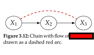
the flow of association and causation in DAGs. We can understand this flow in general DAGs by understanding the flow in the minimal building blocks of graphs. The minimal building blocks of DAGs consist of chains (Figure 3.9a), forks (Figure 3.9b), immoralities (Figure 3.9c), two unconnected nodes (Figure 3.10), and two connected nodes (Figure 3.11)

By “flow of association,” we mean whether any two nodes in a graph are associated or not associated. Another way of saying this is whether two nodes are (statistically) dependent or (statistically) independent.

Additionally, we will study whether two nodes are conditionally independent or not.

Answer: association