Edited, memorised or added to reading queue
on 10-Nov-2016 (Thu)
|
Subject 1. The Nature of Statistics
#quantitative-methods-basic-concepts #statistics
Statistics can refer to numerical data (e.g., a company's average revenue for the past 20 years). It can also refer to methods of collecting, classifying, analyzing, and interpreting numerical data. Statistical methods provide a powerful set of tools for making decisions in business and other fields.
Statistics involves two different processes:
We use statistical methods to analyze the results of data. Since the amount of information available may be vast, it may be extremely time-consuming and expensive to collect all the necessary data. For instance, suppose we are interested in the durability of tennis balls. Theoretically, in order to carry out an accurate assessment, we would need to collect large quantities of all different makes of tennis balls from all over the world. Clearly, this is not practical; aside from taking up lots of time, it would be cost-prohibitive to purchase all the balls we would need for our study. A more practical solution would be to use a sample. A population consists of an entire set of objects, observations, or scores that have something in common. It comprises every possible member of the specified group. In our example above, the population of tennis balls consists of every tennis ball that has ever been manufactured anywhere in the world. This is a huge number of tennis balls. Another example of a population would be all males between the ages of 15 and 18. A sample is a subset of a population. The sample is comprised of some of the members of the population. Since it is usually impractical (or too expensive or time-consuming) to test every member of a population, using data gathered from a sample of the population is typically the best approach available for describing that population. In our example above, a sample might be a selection of 1,000 tennis balls of various makes collected from different sources. It would be a virtually impossible task to collect every possible tennis ball in the world; this same size provides a manageable number to work with as well as a substantial amount of possible data. Before we move on, there are several points worth noting:
|
| status | not read | reprioritisations | ||
|---|---|---|---|---|
| last reprioritisation on | suggested re-reading day | |||
| started reading on | finished reading on |
|
Subject 4. Measures of Center Tendency
#has-images #quantitative-methods-basic-concepts #statistics
Measures of central tendency specify where data are centered. They attempt to use a typical value to represent all the observations in the data set.
Population Mean The population mean is the average for a finite population. It is unique; a given population has only one mean.
 where:
Sample Mean The sample mean is the average for a sample. It is a statistic and is used to estimate the population mean.
 where n = the number of observations in the sample Arithmetic Mean The arithmetic mean is what is commonly called the average. The population mean and sample mean are both examples of the arithmetic mean.
This is the most widely used measure of central tendency. When the word "mean" is used without a modifier, it can be assumed to refer to the arithmetic mean. The mean is the sum of all scores divided by the number of scores. It is used to measure the prospective (expected future) performance (return) of an investment over a number of periods.
The arithmetic mean has the following disadvantages:
Geometric Mean
 The geometric mean has three important properties:
It is typically used when calculating returns over multiple periods. It is a better measure of the compound growth rate of an investment. When returns are variable by period, the geometric mean will always be less than the arithmetic mean. The more dispersed the rates of returns, the greater the difference between the two. This measurement is not as highly influenced by extreme values as the arithmetic mean. Weighted Mean The weighted mean is computed ... |
| status | not read | reprioritisations | ||
|---|---|---|---|---|
| last reprioritisation on | suggested re-reading day | |||
| started reading on | finished reading on |
Flashcard 1417556397324
| status | not learned | measured difficulty | 37% [default] | last interval [days] | |||
|---|---|---|---|---|---|---|---|
| repetition number in this series | 0 | memorised on | scheduled repetition | ||||
| scheduled repetition interval | last repetition or drill |
Flashcard 1417558232332
| status | not learned | measured difficulty | 37% [default] | last interval [days] | |||
|---|---|---|---|---|---|---|---|
| repetition number in this series | 0 | memorised on | scheduled repetition | ||||
| scheduled repetition interval | last repetition or drill |
Flashcard 1417560067340
-significant anemia
-carboxyhemoglobin
(decreased uterine blood flow)
-hypotension
-regional anesthesia
-maternal poisoning
(chr maternal conditions)
-vasculopathies (SLE, T1DM, chr HTN)
-antiphospholipid syndrome
| status | not learned | measured difficulty | 37% [default] | last interval [days] | |||
|---|---|---|---|---|---|---|---|
| repetition number in this series | 0 | memorised on | scheduled repetition | ||||
| scheduled repetition interval | last repetition or drill |
Flashcard 1417561902348
-hyperstimulation d/t oxytocin/prostaglandins/normal labour
-placental abruption
(uteroplacental dysfn)
-placental abruption
-placental infarction/dysfn marked by oligohydramnios/abn doppler studies
-chorioamnionitis
| status | not learned | measured difficulty | 37% [default] | last interval [days] | |||
|---|---|---|---|---|---|---|---|
| repetition number in this series | 0 | memorised on | scheduled repetition | ||||
| scheduled repetition interval | last repetition or drill |
Flashcard 1417563737356
-oligohydramnios
-cord prolapse/entanglement
-decreased fetal oxygen carrying capability
-significant anemia (isoimmunization, fetomaternal bleed)
-carboxyhemoglobin (smokers)
| status | not learned | measured difficulty | 37% [default] | last interval [days] | |||
|---|---|---|---|---|---|---|---|
| repetition number in this series | 0 | memorised on | scheduled repetition | ||||
| scheduled repetition interval | last repetition or drill |
Flashcard 1417565572364
-neonatal neurologic sequelae (hypotonia, seizures, coma)
-evidence of multi-organ system dysfn in the immediate neonatal period
-umbilical cord arterial pH <7.0 and base deficit > 16 mmol/L
| status | not learned | measured difficulty | 37% [default] | last interval [days] | |||
|---|---|---|---|---|---|---|---|
| repetition number in this series | 0 | memorised on | scheduled repetition | ||||
| scheduled repetition interval | last repetition or drill |
Flashcard 1417567407372
| status | not learned | measured difficulty | 37% [default] | last interval [days] | |||
|---|---|---|---|---|---|---|---|
| repetition number in this series | 0 | memorised on | scheduled repetition | ||||
| scheduled repetition interval | last repetition or drill |
Flashcard 1417569242380
• Drug effects
• Maternal position
• Umbilical cord occlusion
• Fetal hypoxia
• Fetal vagal stimulation (head compression)
• Fetal hypothermia
• Fetal acidosis
• Fetal cardiac conduction or structural defect
| status | not learned | measured difficulty | 37% [default] | last interval [days] | |||
|---|---|---|---|---|---|---|---|
| repetition number in this series | 0 | memorised on | scheduled repetition | ||||
| scheduled repetition interval | last repetition or drill |
|
#obgyn
respiratory acidosis (in preg) occurs in vessels when CO2 transport from fetus to placenta is disrupted (e.g. cord compression). It's a part of normal delivery.
|
| status | not read | reprioritisations | ||
|---|---|---|---|---|
| last reprioritisation on | suggested re-reading day | |||
| started reading on | finished reading on |
Flashcard 1417571077388
| status | not learned | measured difficulty | 37% [default] | last interval [days] | |||
|---|---|---|---|---|---|---|---|
| repetition number in this series | 0 | memorised on | scheduled repetition | ||||
| scheduled repetition interval | last repetition or drill |
Open it
respiratory acidosis (in preg) occurs in vessels when CO2 transport from fetus to placenta is disrupted (e.g. cord compression). It's a part of normal delivery.
Flashcard 1417572650252
| status | not learned | measured difficulty | 37% [default] | last interval [days] | |||
|---|---|---|---|---|---|---|---|
| repetition number in this series | 0 | memorised on | scheduled repetition | ||||
| scheduled repetition interval | last repetition or drill |
Open it
respiratory acidosis (in preg) occurs in vessels when CO2 transport from fetus to placenta is disrupted (e.g. cord compression). It's a part of normal delivery.
|
#obgyn
Metabolic acidosis (in preg) develops as a result of fetal hypoxia that causes the fetus to shift to anaerobic metabolism to maintain positive energy balance. Metabolic acidosis is generated in hypoxic tissues, takes longer to develop and disappear, and has the potential to cause significant fetal damage.
|
| status | not read | reprioritisations | ||
|---|---|---|---|---|
| last reprioritisation on | suggested re-reading day | |||
| started reading on | finished reading on |
Flashcard 1417575533836
| status | not learned | measured difficulty | 37% [default] | last interval [days] | |||
|---|---|---|---|---|---|---|---|
| repetition number in this series | 0 | memorised on | scheduled repetition | ||||
| scheduled repetition interval | last repetition or drill |
Open it
Metabolic acidosis (in preg) develops as a result of fetal hypoxia that causes the fetus to shift to anaerobic metabolism to maintain positive energy balance. Metabolic acidosis is generated in hypoxic tissues, takes longer to develop and disappear, a
Flashcard 1417577106700
| status | not learned | measured difficulty | 37% [default] | last interval [days] | |||
|---|---|---|---|---|---|---|---|
| repetition number in this series | 0 | memorised on | scheduled repetition | ||||
| scheduled repetition interval | last repetition or drill |
Open it
Metabolic acidosis (in preg) develops as a result of fetal hypoxia that causes the fetus to shift to anaerobic metabolism to maintain positive energy balance. Metabolic acidosis is generated in hypoxic tissues, takes longer to develop and disappear, and has the potential to cause significant fetal damage.
Flashcard 1417578679564
| status | not learned | measured difficulty | 37% [default] | last interval [days] | |||
|---|---|---|---|---|---|---|---|
| repetition number in this series | 0 | memorised on | scheduled repetition | ||||
| scheduled repetition interval | last repetition or drill |
Open it
Metabolic acidosis (in preg) develops as a result of fetal hypoxia that causes the fetus to shift to anaerobic metabolism to maintain positive energy balance. Metabolic acidosis is generated in hypoxic tissues, takes longer to develop and disappear, and has the potential to cause significant fetal damage.
Flashcard 1417580252428
| status | not learned | measured difficulty | 37% [default] | last interval [days] | |||
|---|---|---|---|---|---|---|---|
| repetition number in this series | 0 | memorised on | scheduled repetition | ||||
| scheduled repetition interval | last repetition or drill |
Open it
<head>Metabolic acidosis (in preg) develops as a result of fetal hypoxia that causes the fetus to shift to anaerobic metabolism to maintain positive energy balance. Metabolic acidosis is generated in hypoxic tissues, takes longer to develop and disappear, and has the potential to cause significant fetal damage.<html>
Flashcard 1417581825292
| status | not learned | measured difficulty | 37% [default] | last interval [days] | |||
|---|---|---|---|---|---|---|---|
| repetition number in this series | 0 | memorised on | scheduled repetition | ||||
| scheduled repetition interval | last repetition or drill |
Open it
s a result of fetal hypoxia that causes the fetus to shift to anaerobic metabolism to maintain positive energy balance. Metabolic acidosis is generated in hypoxic tissues, takes longer to develop and disappear, and has the potential to cause <span>significant fetal damage.<span><body><html>
Flashcard 1417584708876
• Fetal: infection, prolonged fetal activity, chronic hypoxemia, cardiac abnormality, congenital anomalies, anemia
| status | not learned | measured difficulty | 37% [default] | last interval [days] | |||
|---|---|---|---|---|---|---|---|
| repetition number in this series | 0 | memorised on | scheduled repetition | ||||
| scheduled repetition interval | last repetition or drill |
Flashcard 1417587330316
| status | not learned | measured difficulty | 37% [default] | last interval [days] | |||
|---|---|---|---|---|---|---|---|
| repetition number in this series | 0 | memorised on | scheduled repetition | ||||
| scheduled repetition interval | last repetition or drill |
|
#obgyn
Early decel (FHR) is reflex vagal response due to head compression; not normally associated with fetal acidemia
|
| status | not read | reprioritisations | ||
|---|---|---|---|---|
| last reprioritisation on | suggested re-reading day | |||
| started reading on | finished reading on |
Flashcard 1417589165324
| status | not learned | measured difficulty | 37% [default] | last interval [days] | |||
|---|---|---|---|---|---|---|---|
| repetition number in this series | 0 | memorised on | scheduled repetition | ||||
| scheduled repetition interval | last repetition or drill |
Open it
Early decel (FHR) is reflex vagal response due to head compression; not normally associated with fetal acidemia
Flashcard 1417590738188
| status | not learned | measured difficulty | 37% [default] | last interval [days] | |||
|---|---|---|---|---|---|---|---|
| repetition number in this series | 0 | memorised on | scheduled repetition | ||||
| scheduled repetition interval | last repetition or drill |
Open it
Early decel (FHR) is reflex vagal response due to head compression; not normally associated with fetal acidemia
Flashcard 1417592311052
| status | not learned | measured difficulty | 37% [default] | last interval [days] | |||
|---|---|---|---|---|---|---|---|
| repetition number in this series | 0 | memorised on | scheduled repetition | ||||
| scheduled repetition interval | last repetition or drill |
Open it
Early decel (FHR) is reflex vagal response due to head compression; not normally associated with fetal acidemia
Flashcard 1417595194636
| status | not learned | measured difficulty | 37% [default] | last interval [days] | |||
|---|---|---|---|---|---|---|---|
| repetition number in this series | 0 | memorised on | scheduled repetition | ||||
| scheduled repetition interval | last repetition or drill |
Flashcard 1417597029644
If abnormal variable decels, may be associated with fetal acidemia
| status | not learned | measured difficulty | 37% [default] | last interval [days] | |||
|---|---|---|---|---|---|---|---|
| repetition number in this series | 0 | memorised on | scheduled repetition | ||||
| scheduled repetition interval | last repetition or drill |
Flashcard 1417598864652
| status | not learned | measured difficulty | 37% [default] | last interval [days] | |||
|---|---|---|---|---|---|---|---|
| repetition number in this series | 0 | memorised on | scheduled repetition | ||||
| scheduled repetition interval | last repetition or drill |
|
Subject 1. Types of Markets
#cfa #cfa-level-1 #economics #microeconomics #reading-13-demand-and-supply-analysis-introduction
A market is any arrangement that enables buyers and sellers to get information and do business with each other. A competitive market is a market that has many buyers and many sellers so that no single buyer or seller can influence prices.
Broadly speaking there are two types of markets:
The demand for a factor exists because there is a demand for goods that the resource helps to produce. The demand for each factor is thus a derived demand; it is derived from the demand of consumers for products. For example, engineers are needed to design cars. A car manufacturer's demand for engineers thus depends entirely upon the demand for cars. The demand for engineers is a derived demand. |
| status | not read | reprioritisations | ||
|---|---|---|---|---|
| last reprioritisation on | suggested re-reading day | |||
| started reading on | finished reading on |
|
The Demand Function and the Demand Curve
#demand-and-supply #has-images #microeconomics
The demand function represents buyers' behavior.
 Prices influence consumers' purchase decisions. The demand function can be depicted as a negatively sloped demand curve.
Therefore, there is an inverse relationship between the price of a good and the amount that consumers are willing to buy. The demand curve normally slopes downward. It tells the analyst the quantity that consumers are willing to buy for each possible price when all other influences on consumers' planned purchases remain the same. Example 1 Refer to the graph below. What is the quantity of cassettes demanded when their price is $4.00 per week?
 Answer: Two cassettes per week. The demand curve tells how much is demanded at each price. To determine the quantity demanded, find $4.00 on the vertical axis and read across until you meet the demand curve. Then read the quantity from the horizontal axis. When any factor that influences buying plans, other than the price of the good, changes, there is a change in demand for that good. When the quantity of the good that people plan to buy changes at each and every price, there is a new demand curve. These factors include changes in income, number of consumers in the market, changes in the price of a related good, etc. Example 2 Assume the graph below reflects demand in the automobile market. Which arrow best captures the impact of increased consumer income on the automobile market?
 Answer: D. Income is a shift factor of demand. An increase in income increases the number of automobiles demanded at each price. Therefore demand has shifted to the right.
A Change in the Quantity Demanded Versus a Change in Demand The demand curve isolates the impact of price on the amount of a product purchased.
Example 3 Refer to the graph below. Consumers began purchasing more of a product due to a decrease in price. Which arrow best represents this statement?
 Answer: C. A change in price causes a movement along the demand curve. When price falls, the movement is downward and to the right. The Supply Function and ... |
| status | not read | reprioritisations | ||
|---|---|---|---|---|
| last reprioritisation on | suggested re-reading day | |||
| started reading on | finished reading on |
|
Subject 3. Market Equilibrium
#cfa #cfa-level-1 #economics #has-images #microeconomics #reading-13-demand-and-supply-analysis-introduction #subject-3-market-equilibrium
Aggregate Demand and Aggregate Supply
An aggregate demand curve is simply a schedule that shows amounts of a product that buyers collectively desire to purchase at each possible price level. An aggregate supply curve is simply a curve showing the amounts of a product that all firms will produce at each price level. Example 1 Refer to the graph below. What is the market quantity that would be supplied at a price of $2.00?
 Market quantity is the sum of individual quantities supplied at each price. At a price of $2.00, Ann supplies 4, Barry supplies 3, and Charlie supplies 0. The market supply is 7. Market Equilibrium Equilibrium is a state in which conflicting forces are in balance. In equilibrium, it will be possible for both buyers and sellers to realize their goals simultaneously. The following graph depicts the market supply and demand for concert tickets at Madison Square Garden in New York City.
 Equilibrium price and quantity are where the supply and demand curves intersect. Draw a horizontal line from the intersection to the price axis. This is equilibrium price: $60. Draw a vertical line from the intersection to the quantity axis. This is equilibrium quantity: 300. It is equilibrium because quantity demanded equals quantity supplied at $60 per ticket. At this price, there is neither surplus (excess supply) nor shortage (excess demand), so there is no downward or upward pressure for the price to change. Surplus will push prices downward towards equilibrium.

Similarly, shortages push prices upward towards equilibrium. Because the price rises if it is below equilibrium, falls if it is above equilibrium, and remains constant if it is at equilibrium, the price is pulled toward equilibrium and remains there until some event changes the equilibrium. We refer to such an equilibrium as being stable because whenever price is disturbed away from the equilibrium, it tends to converge back to that equilibrium. An unstable equilibrium is an equilibrium that is not restored if disrupted by an external force. While most equilibria studied in economics are of the stable variety, a few cases of unstable equilibria do emerge from time to time, in limited circumstances. |
| status | not read | reprioritisations | ||
|---|---|---|---|---|
| last reprioritisation on | suggested re-reading day | |||
| started reading on | finished reading on |
|
Subject 4. Auctions
#cfa #cfa-level-1 #economics #microeconomics #reading-13-demand-and-supply-analysis-introduction #subject-4-auctions
Auctions can be used to arrive at equilibrium price.
Auctions can be classified as one of two types:
There are also many different methods for auctioning items:
The winner's curse means that the winner of an auction will frequently have bid too much for the auctioned item: you win, you lose money, and you curse. A Dutch auction share repurchase is when a company agrees to buy back a fixed amount of its outstanding shares within a certain price range. Offers come in from investors who specify the price within the given range at which they'll sell their shares. The company then buys back the shares of those who bid the lowest first and continues on up the line until they have bought back the amount that they said they would. The U. S. Treasury security auctions are conducted using the single-price auction method. All successful competitive bidders and all noncompetitive bidders are awarded securities at the price equivalent to the highest rate or yield of accepted competitive tenders. |
| status | not read | reprioritisations | ||
|---|---|---|---|---|
| last reprioritisation on | suggested re-reading day | |||
| started reading on | finished reading on |
|
Subject 5. Consumer Surplus, Producer Surplus, and Total Surplus
#cfa #cfa-level-1 #economics #has-images #microeconomics #reading-13-demand-and-supply-analysis-introduction
Consumer Surplus
Consumer surplus is the area below the demand curve but above the actual price paid. It is the difference between the amount consumers are willing to pay and the amount they have to pay for a good. Consider the market for a good.


Lower market prices increase the amount of consumer surplus in the market. Producer Surplus Producer surplus is the difference between the minimum supply price, represented by the supply curve, and the actual sales price.
Example
 The actual selling price of bananas is $9 per kg. Now imagine that there are only 10,000 kg bananas being supplied at the moment. The marginal cost per kg is only $3 but the selling price is $9. So there is an additional $6 per kg being raised. This is the producer surplus per kg. The total producer surplus when 10,000 kg are produced is thus $60,000. Due to the surplus, more producers enter the market and another 10,000 kg are produced, so there are now 20,000 kg of bananas on the market. The marginal costs of producing this additional 10,000 kg have risen to $4. Producer surplus is not the same as profit. Remember that profit is the return that accrues to owners of a firm and is the difference between sales revenue and total (not marginal) costs of production. Total Surplus The following figure shows that a competitive market creates an efficient allocation of resources at equilibrium.

|
| status | not read | reprioritisations | ||
|---|---|---|---|---|
| last reprioritisation on | suggested re-reading day | |||
| started reading on | finished reading on |
|
Subject 6. Market Interference: The Negative Impact on Total Surplus
#cfa #cfa-level-1 #economics #has-images #microeconomics #reading-13-demand-and-supply-analysis-introduction
The equilibrium price set by the market mechanism is often deemed to be unfair: buyers complain that the price is too high, while sellers believe that it is too low. In such cases, the government may regulate the price of the good or service. This is known as price control. A price control is a government-mandated price that may either be greater or less than the market equilibrium price. Price ceilings and floors are two types of price controls.
A Price Ceiling A price ceiling is a legal restriction that prohibits exchanges at prices greater than a designated price: the ceiling price. Price ceilings are usually imposed when the equilibrium price is considered too high to be fair. A typical price ceiling results in a lower price than market forces would produce. A shortage will result in a situation in which the quantity demanded by consumers exceeds the quantity supplied by producers at the existing price. A typical example of a price ceiling is a "rent ceiling," implemented by over 200 U.S. cities. If the rent ceiling is set above the equilibrium rent, it has no effect. The market works as if there were no ceiling. But if the rent ceiling is set below the equilibrium rent, it has powerful effects.
 If a rent ceiling is set below the equilibrium price P0, for example, at P1, there is a reduction in the quantity that producers are willing to supply qs and an increase in the quantity that consumers demand qd relative to the original equilibrium quantity q. Because the legal price cannot eliminate the shortage, other mechanisms operate. For example, a black market is an illegal market that operates alongside a legal market in which a price ceiling or other restriction has been imposed. A shortage of housing creates a black market in housing. Illegal arrangements are made between renters and landlords at rents above the rent ceiling - and generally above what the rent would have been in an unregulated market. A rent ceiling leads to an inefficient use of resources. The quantity of rental housing is less than the efficient quantity and there is a deadweight loss.
 A rent ceiling decreases the quantity of rental housing, shrinks the total producer and consumer surplus by using resources such as search activity, and creates a deadweight loss. It also transfers part of the producer surplus from producers to consumers. The consumer surplus becomes the green area + the pink area. A Price Floor A price floor is a minimum price that can be legally charged. It usually fixes the price of a good or resource above the market equilibrium level. Price floors are usually imposed when the equilibrium price is considered too low to be fair. Agricultural price supports and minimum wage legislation are examples of price floors.
 If a price floor is set above the equilibrium price, p0, for example, at p1, there is a reduction in quantity demanded from q0 to qd, whilst the quantity supplied increases from q0 to qs. The result is a surplus of qs-qd. Example 1 Refer to the graph below. A price floor set by the government would be binding and cause the greatest distortion in the market if it were established at what price?
 |
| status | not read | reprioritisations | ||
|---|---|---|---|---|
| last reprioritisation on | suggested re-reading day | |||
| started reading on | finished reading on |
|
Subject 7. Demand Elasticities
#cfa #cfa-level-1 #economics #has-images #microeconomics #reading-13-demand-and-supply-analysis-introduction
Elasticity means "responsiveness." The elasticity of demand measures the responsiveness of the quantity demanded of a product to changes in any of the factors that affect demand. Analysts are interested in knowing how much the quantity demanded will rise or fall for a given change in price or income.
Price elasticity of demand is the percentage change in the quantity of a product demanded divided by the percentage change in the price causing the change in quantity. It indicates the degree of consumer response to variation in price. Specifically, it tells the analyst the percentage change in the quantity demanded for a good caused by a 1% increase in the price of that good.
 The change in price is expressed as a percentage of the average price - the average of the initial and new price, and the change in the quantity demanded is expressed as a percentage of the average quantity demanded - the average of the initial and new quantity. Using the average price and average quantity, the same elasticity value is obtained regardless of whether the price rises or falls. The measure is units-free because it is a ratio of two percentage changes and the percentages cancel each other out. Changing the units of measurement of price or quantity leave the elasticity value the same. Because a change in price causes the quantity demanded to change in the opposite direction, this ratio is always negative, although economists always ignore the sign and simply use the absolute value. It is the magnitude, or absolute value, of the measure that reveals how responsive the quantity change has been to a price change. Example 1 A Pizza Hut store can sell 50 pizzas per day at $7 each or 70 pizzas per day at $6 each. The price elasticity is: [(50 - 70)/60] / [(7 - 6) / 6.5] = -2.17. Own-Price Elasticity of Demand Demand can be inelastic, unit elastic, or elastic, and can range from zero to infinity. (Note: the negative sign is ignored.)
Because elasticity is a relative concept, the elasticity of a straight-line demand curve will differ at each point along the demand curve. Specifically, a straight-line demand curve is more elastic when price is high. Note that the elasticity is not the slope of the demand curve. Elasticity is used since it is independent of the units of measure. Example 2 Refer to the graph below. Which of the following is true?
 A. Areas C and E are smaller than area A, so demand must be elastic between $10 and $30. B. Areas C and E are smaller than area A, so demand must be inelastic between $10 and $30. C. Area F is smaller than areas B and C, so demand must be inelastic between $10 and $30. Answer: C. Since at $30 the demand is unit elas... |
| status | not read | reprioritisations | ||
|---|---|---|---|---|
| last reprioritisation on | suggested re-reading day | |||
| started reading on | finished reading on |
|
Subject 1. Utility Theory
#cfa #cfa-level-1 #economics #has-images #microeconomics #reading-14-demand-and-supply-analysis-consumer-demand
Utility refers to the total satisfaction received by a person from consuming a good or service.
Utility theory is a quantitative model of consumer preferences and is based on the above axioms. Consumer preferences can be represented by an ordinal utility function:
 This is a mathematical expression that shows the relationship between utility values and every possible bundle of goods. This ordinal - not cardinal - utility captures only ranking and not strength of preferences. |
| status | not read | reprioritisations | ||
|---|---|---|---|---|
| last reprioritisation on | suggested re-reading day | |||
| started reading on | finished reading on |
|
Subject 2. Indifference Curves
#cfa #cfa-level-1 #economics #has-images #microeconomics #reading-14-demand-and-supply-analysis-consumer-demand
An indifference curve shows the combination of two products that provide an individual with a given level of utility (satisfaction). It is a curve, convex from below, that separates the consumption bundles that are more preferred by an individual from those that are less preferred. The points on the curve represent combinations of goods that are equally preferred by the individual. For example, the bundle at point A of 10 apples and 3 fish provides the same satisfaction as the bundle at point B of 6 apples and 5 fish.

If two consumers have different marginal rates of substitution, they can both benefit from the voluntary exchange of one good for the other. |
| status | not read | reprioritisations | ||
|---|---|---|---|---|
| last reprioritisation on | suggested re-reading day | |||
| started reading on | finished reading on |
|
Subject 3. The Opportunity Set
#cfa #cfa-level-1 #economics #has-images #microeconomics #reading-14-demand-and-supply-analysis-consumer-demand
Assume a world with only two consumer goods, X and Y. Px is the price of good X. X is also the quantity of good X that is purchased by the consumer. Px x X is the consumer's expenditure on good X.
Total expenditure is Px x X + Py x Y. M is the consumer's income or budget. The consumer cannot spend more than her budget allows. Px x X + Py x Y <= M is the consumer's budget constraint. To draw a budget constraint, a line that shows the maximum amount of goods a buyer can purchase with her available funds, you need to know two things: 1) how much money she has, and 2) the prices of the two goods being considered. Assume a consumer has an income of $24. The two goods are rice (price: $2) and beans (price: $3).
 This is the basic budget line. Its slope is an indication of relative prices ($2/$3).
 This is when the price of rice decreases and the consumer can purchase more rice.
 When income doubles, the line will shifts outward, parallel to the original constraint. Similarly, a company's production opportunity set represents the greatest quantity of one product that a company can produce for any given amount of the other good it produces. The investment opportunity set represents the highest return an investor can expect for any given amount of risk undertaken. |
| status | not read | reprioritisations | ||
|---|---|---|---|---|
| last reprioritisation on | suggested re-reading day | |||
| started reading on | finished reading on |
|
Subject 4. Consumer Equilibrium: Maximizing Utility Subject to the Budget Constraint
#cfa #cfa-level-1 #economics #has-images #microeconomics #reading-14-demand-and-supply-analysis-consumer-demand #subject-4-consumer-equilibrium-maximizing-utility-subject-to-the-budget-contraint
The budget constraint line separates consumption bundles that are attainable from those that are unattainable. A consumer will maximise utility by consuming on the highest possible indifference curve (i.e., we assume all income is spent). This is where an indifference curve is tangent to the highest possible budget line.
 A consumer could consume at G, for example, but would be on a higher indifference curve at H. This means that to maximise utility the consumer would consume Q1 of product A and Q2 of product B. The consumer is maximising utility where the budget line and indifference curve are tangent, i.e., MUB/MUA = PB/PA. An Increase in Income An increase in income shifts the budget line out parallel. The new combinations of products that maximise utility can be identified. If this is a normal good, an increase in income increases the quantity demanded.  Inferior goods have a negative income elasticity of demand. Demand falls as income rises.
 |
| status | not read | reprioritisations | ||
|---|---|---|---|---|
| last reprioritisation on | suggested re-reading day | |||
| started reading on | finished reading on |
|
Subject 5. Revisiting the Consumer's Demand Function
#cfa #cfa-level-1 #economics #has-images #microeconomics #reading-14-demand-and-supply-analysis-consumer-demand #subject-5-revisiting-the-consumers-demand-function
Indifference curve analysis lies behind a demand curve. It can be used to examine the effect of price changes and income changes.
If the price of B now falls, the budget line will pivot. The consumer now maximises utility consuming Q3 of product A and Q4 of product B. The fall in the price of product B has led to an increase in the quantity demanded of Q2Q4. This can be shown on a demand curve.
 There are two different phenomena underlying a consumer's response to a price drop:
The substitution and income effects will generally work in the same direction, causing consumers to purchase more as the price falls and less as the price rises. The indifference curve can be used to separate these two effects. In the case of a normal good, higher real income leads to an increase in quantity demanded; this complements the increase due to the substitution effect. This change is shown in the diagram below.
 In the case of an inferior product, the income effect leads to a fall in the quantity demanded, which will work against the substitution effect. In the following diagram the substitution effect is Q2 Q5; the income effect is Q5 Q4. However, the substitution effect outweighs the income effect and overall the quantity demanded rises. The overall change in quantity demanded results in an increase of Q2 Q4. This means the demand curve is downward-sloping, because a price fall increases the quantity demanded.
 When a good is inferior and the income effect outweighs the substitution effect, it is called a Giffen good. This is, however, unlikely, because the substitution effect is almost always stronger than the income effect.


 Another exception is the case where an increase in price causes an increase in demand. This results in an upward-sloping demand curve, and... |
| status | not read | reprioritisations | ||
|---|---|---|---|---|
| last reprioritisation on | suggested re-reading day | |||
| started reading on | finished reading on |
|
Subject 1. Types of Profit Measures
#cfa #cfa-level-1 #economics #has-images #microeconomics #reading-15-demand-and-supply-analysis-the-firm
Accounting Profit
Accounting profit is the profit used by accountants to determine a firm's net income.
Economic profit equals a firm's total revenue minus its total opportunity costs of production.
The total opportunity costs include both explicit and implicit costs of all the resources used by a firm. Implicit opportunity cost is the unearned or nominal profit that the resource-owner did not make from investing in the next best alternative. As a result, you can have a significant accounting profit with little to no economic profit. Example Suppose a person uses his own resources, land, capital, and time in the production of goods. The opportunity costs of these resources are shown below: Accounting Profit = $55,000 Entrepreneur's own forgone salary = $40,000 Foregone interest on capital = $1,000 Foregone rent = $2,000 Economic Profit = 55,000 - 40,000 - 1,000 - 2,000 = $12,000 For publicly traded corporations, economic profit is accounting profit - required return on equity capital. When economic profit is zero, a firm's accounting profit becomes normal profit, which is effectively the total implicit opportunity cost.
When a firm's total revenues are just equal to its total costs, its economic profit is zero, but it still makes accounting profit. Zero economic profit does not mean that the firm is about to go out of business. Instead, it just indicates that the owners are receiving exactly the market (normal) rate of return on their investment. Economic Rent The total income received by an owner of a factor of production is made up of its economic rent and its opportunity cost.
The following figure illustrates the division of a factor income into economic rent and opportunity cost.
 The portion of income comprised of economic rent depends upon the elasticity of supply for the factor.
|


| status | not read | reprioritisations | ||
|---|---|---|---|---|
| last reprioritisation on | suggested re-reading day | |||
| started reading on | finished reading on |
|
Subject 2. Total, Average, and Marginal Revenue
#cfa #cfa-level #economics #has-images #microeconomics #reading-15-demand-and-supply-analysis-the-firm
Revenue is the income generated from the sale of output in product markets.
In a perfectly competitive market, each firm is a price taker. Since each unit of output sold by a price taker is sold at the market price, the MR for each unit is also equal to the market price, i.e., P = MR.
 Under imperfect competition, a firm's marginal revenue is always less than the price of its good. Why? As the firm reduces price in order to expand output and sales, there will be two conflicting influences on total revenue.
These two conflicting forces will result in marginal revenue - the change in total revenue - that is less than the sales price of the additional units. Thus, the marginal revenue curve of the firm will always lie below the firm's demand curve, which is also the market's demand curve.
 TR is maximized when MR = 0. |


| status | not read | reprioritisations | ||
|---|---|---|---|---|
| last reprioritisation on | suggested re-reading day | |||
| started reading on | finished reading on |
|
Subject 3. Cost Measures
#cfa #cfa-level #economics #has-images #microeconomics #reading-15-demand-and-supply-analysis-the-firm
Factors of Production
A firm is an institution that hires factors of production and organizes them to produce and sell goods and services. Such factors include land, labor, capital, and materials. The total product curve shows how total product changes with the quantity of variable input employed.
 As more and more units of a variable resource are combined with a fixed amount of other resources, employment of additional units of the variable resource will eventually increase output only at a decreasing rate. Once diminishing returns are reached, it will take successively larger amounts of the variable factor to expand output by one unit. The law of diminishing returns basically explains the old adage: "too many cooks spoil the broth," or too much of a good thing is bad. Total, Average, Marginal, Fixed, and Variable Costs To produce more output in the short run, the firm must employ more variable inputs, which means that it must increase its costs. In the short run, a firm's total costs (TC) can be broken down into two categories: fixed costs and variable costs (TC = TFC + TVC). Which costs are fixed and which costs are variable depends on the time horizon being dealt with. For a short time horizon, most costs are fixed. For a long time horizon, all costs are variable.
 Over the output range with increasing marginal returns, marginal cost falls as output increases. Once a firm confronts diminishing returns, larger and larger additions of the variable factor are required to expand output by one unit. This will cause marginal cost (MC) to rise. As MC continues to increase, eventually it w... |


| status | not read | reprioritisations | ||
|---|---|---|---|---|
| last reprioritisation on | suggested re-reading day | |||
| started reading on | finished reading on |
|
Subject 4. Shutdown Analysis
#cfa #cfa-level #economics #has-images #microeconomics #reading-15-demand-and-supply-analysis-the-firm
For a price taker (a firm in a perfectly competitive market):
However, maximum profit is not always a positive economic profit. In the short run, the firm might break even (making a zero economic profit), make an economic profit, or incur an economic loss. 1. If the price equals minimum average total cost, the firm breaks even and makes a normal profit. 2. The ATC of producing each of q2 units is labeled as c1.
 c1BAP indicates the economic profit being made by this firm. The firm is making a profit since the price per unit exceeds the ATC per unit and the total revenue exceeds the total costs. 3. What would happen to profits if the price fell to below the ATC curve?
 The firm therefore will produce q1 units of output, as shown where MC = MR. At q1, the firm can only charge P per unit, and yet the ATC per unit is higher, at c2. This means that the firm is making a total economic loss equal to the shaded area, PBAc2, or the distance of c2 to P per unit. If the firm's current sales revenues can cover its variable cost, and the firm anticipates that the lower market price is temporary, it will continue to operate and will face short-run economic losses. It will produce the quantity at which MC = P. This option is better than "shut down" since the firm is able to cover its variable costs and pay some of its fixed costs. If it were to shut down, the firm would lose the entire amount of its fixed costs.
 The shutdown point is the output and price at which the firm just covers its total variable cost.
If the market price is below the firm's average variable cost, a temporary shutdown is preferable to short-run operation. If the firm continues to operate, operating losses merely add to losses resulting from the firm's fixed costs. Shutdown will reduce losses.
 The Firm's Short-Run Supply Curve The price taker that intends to stay in business will maximize profits (or minimize losses) when it produces the output level at which P = MC AND variable costs are covered. At this output level, the price taker can maximize its profits or minimizes its losses. Therefore, the portion of the firm's short-run marginal cost curve that lies above its average variable cost is the short-run curve of the firm.
 In the above graph, if price is below P1, the firm should be shut down. |
| status | not read | reprioritisations | ||
|---|---|---|---|---|
| last reprioritisation on | suggested re-reading day | |||
| started reading on | finished reading on |
|
Subject 5. Economies of Scale and Diseconomies of Scale
#cfa #cfa-level #economics #has-images #microeconomics #reading-15-demand-and-supply-analysis-the-firm
Short-Run Cost and Long-Run Cost
The short-run analysis relates costs to output for a specific size of plant. In the long-run, all resources used by the firm are variable. For each plant size, there is a set of short-run, U-shaped costs curves for MC, AVC, and ATC. This diagram shows the ATC curves of three (of many) possible plant sizes: small, medium, and large.
 Using this information, firms can plan, when in their blueprint stages, the optimal plant size they should be relative to the output they want to produce. For example, if a firm wanted to produce more than Q1 units of output, it would make sense to build a large firm, since costs per unit would be less than they would be with a small or medium firm.
 Long-Run Average Cost Curve To explain this process, imagine the output level Q2. Looking at the relevant costs on the vertical axis, the large firm is far cheaper per unit than both the small and medium-sized firms.
 Thus, should a firm be planning for output in excess of Q1, a large firm should be built. For levels of output between Q0 and Q1, it would be cheaper per unit if the firm was of a medium size.
 The long-run average total cost curve is indicated in black.
 It shows the minimum average cost of producing each output level when the firm is free to choose among all possible plant sizes. It can best be thought of as a planning curve, because it reflects the expected per-unit cost of producing alternative rates of output while plants are still in the blueprint stage. No single plant size could produce the alternative output rates at the costs indicated by the planning curve. In reality, there are an infinite number of firm sizes:
 Economies and Diseconomies of Scale Economies of scale are reductions in the firm's per-unit costs that are associated with the use of large plants to produce a large volume of output. They are present over the initial range of outputs when the long-run ATC curve is falling. There are three reasons why economies of scale exist:
Diseconomies of scale are situations in which the long-run average total costs are greater in larger firms than they are for smaller firms. They are possible: as a firm gets bigger and bigger, bureaucratic inefficiencies may result. Principal-agent problems grow; they are prese... |
| status | not read | reprioritisations | ||
|---|---|---|---|---|
| last reprioritisation on | suggested re-reading day | |||
| started reading on | finished reading on |
|
Subject 6. Profit Maximization
#cfa #cfa-level #economics #has-images #microeconomics #reading-15-demand-and-supply-analysis-the-firm
The goal of each firm is to maximize economic profit, which equals total revenue minus total cost.
Marginal revenue is the addition to total revenue earned by a firm when one more unit of output is sold: MR = ΔTR/ΔQ. Since each unit of output sold by a price taker is sold at the market price, the MR for each unit is also equal to the market price, i.e., P = MR. MR plotted against quantity sold would thus yield the same curve as P plotted against quantity sold (i.e., the demand curve) for the price taker.
  We say that the MR curve of a price taker lies on the demand curve of a price taker.
 There are three approaches to calculating the point of profit maximization in the short run. All three approaches yield the same profit-maximizing quantity of output. MC = MR Approach Produce that quantity of output where: MC = P = MR
Here are two familiar curves: the MC curve and the MR curve of a certain firm. Note that the MC curve clearly illustrates the Law of Diminishing Returns. Given this information, what quantity of output should this profit-maximizing price taker produce?
 What about producing q1 units?
 Can you see that at q1, MR exceeds MC by the distance shown by the arrow? This means that the revenue received from the sale of that unit would exceed the cost of its production, so it would be profitable for the firm to produce that unit. But would the firm be maximizing its profits, or should the firm produce more? What about producing q2 units?
 MR still exceeds MC, shown by the distance of the arrow. This means that the revenue received from the sale of unit q2 also exceeds its cost of production, so the firm would make even more profit if it produced that unit too. But would the firm be maximizing its profits? Could the firm produce still more units? At q3, the MR earned from the sale of the unit is equal to the MC involved in producing the unit, so unit q3 generates neither a profit nor a loss for the firm.
 If the firm produced more than q... |
| status | not read | reprioritisations | ||
|---|---|---|---|---|
| last reprioritisation on | suggested re-reading day | |||
| started reading on | finished reading on |
|
Subject 7. Productivity
#cfa #cfa-level #economics #has-images #microeconomics #reading-15-demand-and-supply-analysis-the-firm
Average product and marginal product, which are derived from total product, are key measures of a firm's productivity.
Law of Diminishing Returns The total product curve shows how total product changes with the quantity of variable input employed.
 As more and more units of a variable resource are combined with a fixed amount of other resources, employment of additional units of the variable resource will eventually increase output only at a decreasing rate. Once diminishing returns are reached, it will take successively larger amounts of the variable factor to expand output by one unit. The law basically explains the old adage: "too many cooks spoil the broth," or too much of a good thing is bad. As a single resource is applied more intensively, the resource eventually tends to accomplish less and less. Essentially, this is a constraint imposed by nature. Let's use labor as the input. Initially, hiring more laborers may mean more productive use of machines, which were underutilized. Output may thus initially increase. After a while, the firm may have hired too many laborers, given the number of machines. There may be overcrowding on the work floor and mistakes may result, causing productivity to fall whilst costs will increase.
 As units of variable input are added to a fixed input, total product will increase, first at an increasing rate and then at a declining rate. This will cause both marginal and average product curves to rise at first and then decline. Note that the marginal product curve intersects the average product curve at its maximum. The smooth curves indicate that the input can be increased by amounts of less than a single unit. Profit Maximization Firms demand labor, amongst other factors, to produce goods and services. The Marginal Revenue Product (MRP) of labor is the change in the total revenue of a firm that results from the employment of one additional unit of labor. The marginal revenue product of an input is equal to its marginal product multiplied by the marginal revenue of the good or service produced: MRP = MP x MR, where
Because of the law of diminishing returns, the marginal product of labor will fall as employment of the labor expands, and thus the marginal revenue product of labor will also fall as employment expands. The firm has two equivalent conditions for maximizing profit. They are:
Why? MRP = W => MP x MR = W => MR = W/MP, since W/MP = MC => MR = MC. This relationship indicates why wage differences across skill categories will tend to reflect product... |
| status | not read | reprioritisations | ||
|---|---|---|---|---|
| last reprioritisation on | suggested re-reading day | |||
| started reading on | finished reading on |
|
Subject 1. Characteristics of Different Market Structures
#cfa #cfa-level #economics #microeconomics #reading-16-the-firm-and-market-structures
A financial analyst must understand the characteristics of market structures to better forecast a firm's future profit stream.
We focus on those characteristics that affect the nature of competition and pricing. They are:
The characteristics of each market structure will be discussed in subsequent subjects of this reading. |
| status | not read | reprioritisations | ||
|---|---|---|---|---|
| last reprioritisation on | suggested re-reading day | |||
| started reading on | finished reading on |
|
Subject 2. Perfect Competition
#cfa #cfa-level-1 #economics #has-images #microeconomics #reading-16-the-firm-and-market-structures
An industry with perfect competition displays the following characteristics:
Perfect competition arises:
The demand analysis in perfectly competitive markets is covered in Reading 13. The supply analysis, optimal price and output, and long-run equilibrium in perfectly competitive markets are covered in Reading 15. In perfect competition, each firm is a price taker. Price takers are sellers who must take the market price in order to sell their products.
This diagram represents the market demand and supply curve for a certain product - for example, eggs.
 As usual, the intersection of the demand and supply curve creates the market price (P) per egg. Now remember that a firm that is a price taker can sell all it wants to at that price, but can sell nothing at a higher price.
 Price takers can sell all their output at the market price, but they are unable to sell any of their output at a price higher than the market price. That is, a price taker faces a horizontal demand curve. Each firm's output is a perfect substitute for the output of the other firms, so the demand for each firm's output is perfectly elastic.
When a perfectly competitive market is in long-run equilibrium:
 Why do firms earn zero economic profit in the long-run equilibrium?
|
| status | not read | reprioritisations | ||
|---|---|---|---|---|
| last reprioritisation on | suggested re-reading day | |||
| started reading on | finished reading on |
|
Subject 3. Monopolistic Competition
#cfa #cfa-level #economics #has-images #microeconomics #reading-16-the-firm-and-market-structures
A monopolistic market is also called a competitive price searcher market.
Characteristics are:
Consider two hamburger companies: McDonald's and Burger King.
The Firm's Short-Run Output and Price Decision As with price takers, monopolistic competitors maximize profits by expanding output to where MR = MC. A firm in monopolistic competition operates much like a single-price monopolist.
 According to the demand curve, the firm can charge P1 per unit.
A firm might incur an economic loss in the short run when P < ATC. Long Run: Zero Economic Profit Whenever firms can freely enter and exit a market, profits and losses play an important role in determining the size of the industry. Economic profits will attract new competitors to the market and economic losses will cause competitors to exit from the market. In the short run, a price searcher may make either economic profits or losses, depending on market conditions. As firms enter the industry, each existing firm loses some of its market share. The demand for its product decreases and the demand curve for its product shifts leftward.
 The decrease in demand decreases the quantity at which MR = MC and lowers the maximum price that the firm can charge to sell... |
| status | not read | reprioritisations | ||
|---|---|---|---|---|
| last reprioritisation on | suggested re-reading day | |||
| started reading on | finished reading on |
|
Subject 4. Oligopoly
#cfa #cfa-level #economics #has-images #microeconomics #reading-16-the-firm-and-market-structures
Literally, oligopoly means "few sellers." This market structure is characterized by:
In short, an oligopoly is competition among the few. Pricing Strategies
A key factor here is the pricing behavior of close rivals, or interdependence between firms. This means that each firm must take into account the likely reactions of other firms in the market when making pricing decisions. Because the reactions of those rivals cannot be determined, the precise price and output that will emerge under an oligopoly cannot be determined. Only a potential range of prices can be indicated. There are three basic pricing strategies. 1. The assumption of pricing interdependence is that firms will match a price reduction and ignore a price increase. The idea is that if a firm raises prices, other firms won't follow, because they won't worry about losing market share to a firm that is raising its prices. However, if the firm lowers its prices, other firms will respond by lowering their prices also, since they don't want to lose market share. The demand curve that a firm believes it faces has a kink at the current price P and quantity Q.
 The kinked demand curve can be thought of as two demand curves.
The kink in the demand curve means that the MR curve is discontinuous at the current quantity - shown by the gap AB in the figure. Fluctuations in MC that remain within the discontinuous portion of the MR curve leave the profit-maximizing quantity and price unchanged. For example, if costs increased so that the MC curve shifted upward from MC0 to MC1, the profit-maximizing price and quantity would not change. The beliefs that generate the kinked demand curve are not always correct and firms can figure out this fact. If MC increases enough, all firms raise their prices and the kink vanishes. 2. The assumption of the Cournot... |
| status | not read | reprioritisations | ||
|---|---|---|---|---|
| last reprioritisation on | suggested re-reading day | |||
| started reading on | finished reading on |
|
Subject 5. Monopoly
#cfa #cfa-level #economics #has-images #microeconomics #reading-16-the-firm-and-market-structures
Literally, monopoly means "single seller." It is a market structure characterized by:
Barriers to entry include legal or natural constraints that protect a firm from potential competitors.
Demand and Supply Analysis A monopoly faces no competition, and as a result there is no product differentiation. It is a price setter, not a price taker like a firm in perfect competition. Because the monopoly is the only seller in the market, the demand for its product is the market demand curve. It is downward-sloping because demand will decline as price increases. Marginal Revenue and Price A monopoly must choose between lower prices with larger quantities sold and higher prices with smaller sales. Although a monopoly can set the price for its products, market forces will determine the quantity sold at alternative prices. To maximize profit, a monopoly must estimate the relationship between price and the quantity of its products demanded. As the monopoly reduces price in order to expand output and sales, there will be two conflicting influences on total revenue.
These two conflicting forces will result in marginal revenue - the change in total revenue - that is less than the sales price of the additional units. Thus, the marginal revenue curve of the monopoly will always lie below the firm's demand curve, which is also the market's demand curve:
The following example illustrates this concept.
 Portico produces beauty soaps.
|
| status | not read | reprioritisations | ||
|---|---|---|---|---|
| last reprioritisation on | suggested re-reading day | |||
| started reading on | finished reading on |
|
Subject 6. Price Discrimination
#cfa #cfa-level #economics #has-images #microeconomics #reading-16-the-firm-and-market-structures
Price discrimination is a practice whereby a seller charges different consumers different prices for the same product or service. It converts consumer surplus into economic profit.
When sellers can segment their market (at a low cost) into groups with differing price elasticities of demand, price discrimination can increase profits. For each group, the seller will maximize profit by equating marginal cost and marginal revenue. The number of units sold also increases because the discounts provided to price-sensitive groups increase the quantity sold more than the higher prices charged the less price-sensitive groups reduce sales. Imagine that the MC per unit for a monopoly is constant at $60, producing a horizontal MC curve, as shown below.
 The firm produces where MC = MR. It thus produces 100 units and charges $200 per unit. Total revenue (price x quantity) for the firm is thus: $200 x 100 = $20,000. Total costs (cost per unit x quantity) are: $60 x 100 = $6,000. Total profit is thus: $20,000 - $6,000 = $14,000. Imagine that this firm is an airline and that it now decides to increase its profits using price discrimination. It identifies two groups of people: businessmen, who are fairly price-inelastic, and students, who are fairly price-elastic (responsive to changes in price). By increasing the price of businessmen's tickets and decreasing the price of student's tickets, it can increase its total revenue and thus increase its profit. The airline starts by doubling the price of businessmen's tickets to $400. By equating the businessmen's MR curve to the MC curve (for simplicity, the MR curve is not shown), the airline finds that the quantity demanded decreases, but by relatively little, given the large increase in price, to 60 tickets.
 Next, it equates MC to the students' MR curve and finds that it can decrease the price of students' tickets from $200 to $150, whilst the quantity demanded increases to 150 tickets. (Note: for simplicity, the students' MR curve is not shown).
 Therefore, the total revenue is as follows: $400 x 60 + $150 x 150 = $46,500. Total costs are: $60 x 60 + $60 x 150 = $12,600. Total profits are thus: $46,500 - $12,600 = $33,900. This is more than the $14,000 profit the firm made in the absence of price discrimination.
 |
| status | not read | reprioritisations | ||
|---|---|---|---|---|
| last reprioritisation on | suggested re-reading day | |||
| started reading on | finished reading on |
|
Subject 7. Identification of Market Structure
#cfa #cfa-level #economics #microeconomics #reading-16-the-firm-and-market-structures
Measuring market power is complicated. Ideally, econometric estimates of the elasticity of demand and supply should be computed. However, because of the lack of reliable data and the fact that elasticity changes over time (so that past data may not apply to the current situation), regulators and economists often use simpler measures.
The N-firm concentration ratio is the percentage of market output generated by the N largest firms in the industry. The ratio is used as an indicator of the relative size of firms in relation to the industry as a whole. It may also assist in determining the market form of the industry. The larger the measure of market concentration, the less competition exists in the industry. The concentration ratio is simple to compute. However, it does not directly quantify market power, meaning it does not take the possibility of entry into account. Another disadvantage is that it ignores mergers among the top market players. The Herfindahl-Hirschman Index (HHI) The Herfindahl-Hirschman index is the sum of the squared market shares of the top N largest firms in the industry.
where Mi is the market share of an individual firm. Suppose there are a total of four firms in a specific industry. Three firms have a 20% share each and one has a 40% market share, H = 0.202 + 0.202 + 0.202 + 0.402 = 0.28. The advantages of the Herfindahl index are that it reflects more firms in the industry and it gives greater weight to the companies with larger market shares. Properties of the Herfindahl index:
Limitations: HHI fails to consider barriers to entry and firm turnover. For example, for some industries, few firms may be currently operating in the market but competition might be fierce, with firms regularly entering and exiting the industry. Even potential entry might be enough to maintain competition. |
| status | not read | reprioritisations | ||
|---|---|---|---|---|
| last reprioritisation on | suggested re-reading day | |||
| started reading on | finished reading on |
|
Subject 1. Gross Domestic Product
#cfa #cfa-level-1 #economics #macroeconomics #reading-17-aggregate-output-and-economic-growth
Gross Domestic Product (GDP) is the total market value of all domestically produced final goods and services for a particular year. Its five key factors are: market value, final goods and services, produced, within a country, during a specific time period.
Government services and household production are estimated and included in the GDP. Activities occurring in the underground economy, although sometimes productive, are not included in GDP. Nominal and Real GDP When comparing GDP across time periods, we confront a problem: the nominal value of GDP may increase as the result of either expansion in the quantities of goods produced or higher prices. Since the former will improve our living standards, we have to adjust the nominal values (nominal GDP, or money values) for the effects of inflation to get real values (real GDP). A price index is used for the adjustment. It measures the cost of purchasing a market basket or bundle of goods at a point in time relative to the cost of purchasing the identical market basket during an earlier reference period (e.g., a base year). Consumer price index (CPI) (not included in the required reading) is an indicator of the general level of prices. It attempts to compare the cost of purchasing the market basket bought by a typical consumer during a specific period with the cost of purchasing the same market basket during an earlier period. The CPI is better at determining how rising prices affect the money income of consumers. The CPI is more widely used for price changes over time. The GDP deflator is a price index that reveals the cost during the current period of purchasing the items included in GDP relative to the cost during a base year. Because the base year is assigned a value of 100, as the GDP deflator takes on values greater than 100, it indicates that prices have risen. It is a broader price index than the CPI since it is better at giving an economy-wide measure of inflation. It is designed to measure the change in the average price of the market basket of goods included in GDP. In addition to consumer goods, the GDP deflator includes prices for capital goods and other goods and services purchased by businesses and governments. The GDP deflator also allows the basket of goods to change as the composition of GDP changes, while the CPI is computed using a fixed basket of goods. We can use the GDP deflator together with nominal GDP to measure the real GDP (GDP in dollars of constant purchasing power). Real GDPi = Nominal GDPi x (GDP Deflator for base year/ GDP Deflator for year i) Suppose the nominal GDPs in 1992 and 2010 were $6244 and $8509 billion dollars, respectively. This amount has increased by 36.3%. The GDP deflator for 1992 and 2010 was 100 and 112.7, respectively. The re... |
| status | not read | reprioritisations | ||
|---|---|---|---|---|
| last reprioritisation on | suggested re-reading day | |||
| started reading on | finished reading on |
|
Subject 2. The Components of GDP and Related Measures
#cfa #cfa-level-1 #economics #macroeconomics #reading-17-aggregate-output-and-economic-growth
GDP is a measure of both output and income. The revenues that firms derive from the sale of goods and services are paid directly to resource suppliers in the form of wages, self-employment income, rents, profits, and interest.
There are two ways of measuring GDP. GDP derived by these two approaches will be equal. The expenditure approach totals the expenditures spent on all final goods and services produced during the year. Under this approach, GDP is a measure of aggregate output. There are four components of GDP under this approach:
GDP can be measured either from the value of the final output or by summing the value added at each stage of the production and distribution process. The sum of the value added by each stage is equal to the final selling price of the good. Under the income approach, GDP is a measure of aggregate income. It is calculated by summing the income payments to resource suppliers and the other costs of producing those goods and services. It includes employee compensation (wages and salaries), self-employment income, rents, profits and interest, etc. Employee compensation is the largest source of income generated by the production of goods and services. Personal income is the total income received by domestic households and non-corporate businesses. It is available for consumption, saving, and payment of personal taxes. Personal disposable income is an individual's available income, after personal taxes are paid, that can be either consumed or saved. |
| status | not read | reprioritisations | ||
|---|---|---|---|---|
| last reprioritisation on | suggested re-reading day | |||
| started reading on | finished reading on |
|
Subject 3. Aggregate Demand
#cfa #cfa-level-1 #economics #has-images #macroeconomics #reading-17-aggregate-output-and-economic-growth
Aggregate demand (AD) is the quantity of goods and services that households, businesses, and foreign customers want to buy at any given level of prices.
The IS Curve GDP = C + I + G + (X - M)
We can also derive the following equation, which shows that domestic saving has three uses: investment, government deficits, and trade surplus: S = I + (G - T) + (X - M), where S is domestic saving. If we combine these relationships together we can derive the IS curve: the combination of GDP (Y) and the real interest rate (i) such that aggregate income/output equals planned expenditures.
 Note that there is an inverse relationship between income and the real interest rate. For example, when interest rates are high, investment falls and therefore Y must fall as well. Note that changes in Y caused by changes in i are reflected as movements along the IS curve. On the other hand, changes in Y that are brought about by factors other than interest rates will cause Y to change, regardless of the level of interest rates in the economy. For example, changes in government purchases will not change the slope but will change the intercepts; in other words, they will cause the IS curve to shift.  The LM Curve The IS curve depicts combinations of interest rates and output that clears markets for goods and services. The IS curve by itself does not pin down the interest rate that prevails in the economy. In order to do so, we look at the money market. The LM curve summarizes all the combinations of income and interest rates that equate money demand and money supply. The quantity theory of money: MV = PY, where V is the velocity of money.
When the money market is in equilibrium, money supply = money demand. The LM curve summarizes all the combinations of income and interest rates that equate money demand and money supply. It is an upward-sloping relationship between i and Y.  Intuitively, we can explain the upward-sloping LM curve as follows: Let's consider some combination of income and interest rates that equates money demand with the money supply set by the Fed. Now suppose there is ... |
| status | not read | reprioritisations | ||
|---|---|---|---|---|
| last reprioritisation on | suggested re-reading day | |||
| started reading on | finished reading on |
|
Subject 4. Aggregate Supply
#cfa #cfa-level-1 #economics #has-images #macroeconomics #reading-17-aggregate-output-and-economic-growth
The aggregate quantity of goods and services supplied depends on three factors: labor (L), capital (K), and the state of technology (T).
The aggregate supply curve (AS) represents the relationship between the quantity of goods and services supplied and the price level. It is important to distinguish between long-run aggregate supply and short-run aggregate supply. The short-run aggregate supply curve typically slopes upward to the right. In the short run, some prices (e.g., rents, wages) are temporarily fixed as the result of prior commitments. Therefore, firms will expand outputs as the price level increases because higher prices will improve profit margins. Short-run equilibrium occurs when the aggregate quantity of goods and services demanded is equal to the aggregate quantity supplied.
 The long-run aggregate supply curve is vertical. In the long run, people have sufficient time to alter their behavior to adjust fully to price changes. The sustainable level of output is determined by a nation's resource base, technology, and the efficiency of its institutional factors. The price level has no effect on a nation's long-run aggregate supply. In long-run equilibrium, current output (Yfull) will equal the economy's potential GDP, the economy is operating at full employment, and the actual rate of unemployment will equal the natural rate of unemployment.  Aggregated demand and supply determine the level of real GDP and the price level of a nation.
 |
| status | not read | reprioritisations | ||
|---|---|---|---|---|
| last reprioritisation on | suggested re-reading day | |||
| started reading on | finished reading on |
|
Subject 5. Shifts in Aggregate Demand and Supply
#cfa #cfa-level-1 #economics #has-images #macroeconomics #reading-17-aggregate-output-and-economic-growth
Factors that Shift Aggregate Demand
At each price level, the AD curve shifts to the right due to changes in C, I, G, and X.
And vice versa. Factors that Shift Aggregate Supply We need to differentiate between the long-run and short-run effects.  Increases in short-run aggregate supply (SRAS) that don't affect long-run aggregate supply are caused by:
And vice versa.
 Long-run supply refers to the economy's long-run production possibilities (maximum rate of sustainable output). Increase in long-run aggregate supply (LRAS) is caused by:
And vice versa. |
| status | not read | reprioritisations | ||
|---|---|---|---|---|
| last reprioritisation on | suggested re-reading day | |||
| started reading on | finished reading on |
|
Subject 6. Equilibrium GDP and Prices
#cfa #cfa-level-1 #economics #has-images #macroeconomics #reading-17-aggregate-output-and-economic-growth
Short-run macroeconomic equilibrium occurs when the quantity of real GDP demanded equals the quantity of real GDP supplied at the point of intersection of the AD curve and the SAS curve. If real GDP is below equilibrium GDP, firms increase production and raise prices, and if real GDP is above equilibrium GDP, firms decrease production and lower prices. These changes bring a movement along the SAS curve towards equilibrium.
In short-run equilibrium, real GDP can be greater than or less than potential GDP. Long-run macroeconomic equilibrium occurs when real GDP equals potential GDP - when the economy is on its LAS curve.
 Note two things:
Long-run equilibrium thus occurs where LAS, AD, and SAS coincide. Economic Growth and Inflation Economic growth occurs because the quantity of labor grows, capital is accumulated, and technology advances, all of which increase potential GDP and bring a rightward shift of the LAS curve. The following figure illustrates economic growth and inflation.
 Inflation occurs because the quantity of money grows faster than potential GDP, which increases aggregate demand by more than long-run aggregate supply. The AD curve shifts rightward faster than the rightward shift of the LAS curve. The Business Cycle The business cycle occurs because aggregate demand and short-run aggregate supply fluctuate.
  Let's look at the inflation gap. An economic boom may be the result of an increase in AD. Starting at long-run equilibrium, an increase in aggregate demand shifts the AD curve rightward.
 The prices of goods and services increase, which in turn induces suppliers to expand output to a level that is unsustainable in the long run (which is why a boom is followed by an economic contraction). That is, firms increase output and prices - a movement along the SRAS curve. Since prices are currently high (P1) and the situation is moving into the long run, people will expect prices to continue to be high. There is an inflationary gap. Stagflation In the resource market, a supply shock such as a drought or high oil prices is reflec... |
| status | not read | reprioritisations | ||
|---|---|---|---|---|
| last reprioritisation on | suggested re-reading day | |||
| started reading on | finished reading on |
|
Subject 7. Economic Growth and Sustainability
#cfa #cfa-level-1 #economics #macroeconomics #reading-17-aggregate-output-and-economic-growth
Economic growth is the sustained expansion of production possibilities measured as the increase in real GDP over a given period. The economic growth rate is the annual percentage change of real GDP. It tells us how rapidly the total economy is expanding.
The standard of living depends on real GDP per person. Real GDP per person is real GDP divided by the population. It grows only if real GDP grows faster than the population grows. The Production Function and Potential GDP
The quantity of real GDP supplied, Y, depends on the quantity of labor, L, the quantity of capital, K, and the state of technology, A (total factor productivity). This equation shows that output depends on inputs and the level of technology.
The law of diminishing returns: As the quantity of one input increases with the quantities of all other inputs remaining the same, output increases but by ever smaller increments. As capital per hour of labor rises, output rises (the marginal product of capital is positive) but output rises less at high levels of capital than at low levels. This is the key explanation of why the economy reaches a steady state rather than growing endlessly. Convergence is the process of one economy catching up with another economy. According to the neoclassical growth theory, countries with a low level of capital would have a higher marginal product of capital because of diminishing returns and hence attract more investment and grow faster. Growth in Y = Growth in technology + WL (growth in labor) + WC (growth in capital) where WL and WC = 1 - WL are the shares of labor and capital in GDP. Sources of Economic Growth There are five important sources of growth for an economy:
Measures of Sustainable Growth Labor productivity is the quantity of real GDP produced by an hour of labor. The growth of labor productivity depends on physical capital growth, human capital growth, and technology advances.
Potential growth rate = Long-term growth rate of labor force + Long-term labor productivity growth rate |
| status | not read | reprioritisations | ||
|---|---|---|---|---|
| last reprioritisation on | suggested re-reading day | |||
| started reading on | finished reading on |
|
Subject 1. The Business Cycle and its Phases
#cfa #cfa-level-1 #economics #has-images #macroeconomics #reading-18-understanding-business-cycles
The business cycle is the fluctuations in the general level of economic activity as measured by such variables as the rate of unemployment and changes in real GDP. Periods of growth in real output and other aggregate measures of economic activity followed by periods of decline are distinguishing characteristics of business cycles. A complete business cycle is represented by A to G in the diagram below:

|
| status | not read | reprioritisations | ||
|---|---|---|---|---|
| last reprioritisation on | suggested re-reading day | |||
| started reading on | finished reading on |
|
Subject 2. Theories of the Business Cycle
#cfa #cfa-level-1 #economics #macroeconomics #reading-18-understanding-business-cycles
We consider a few fundamentally different theories of the business cycle.
Neoclassicial and Austrian Schools - Self-Correcting Economy The neoclassical economists assumed that the economy would not operate with real GDP (Y) away from the level of natural real GDP (YN) for any length of time; if Y < YN, then firms would be producing below capacity, and would tend to cut nominal wages and prices, which would continue until YN was again reached. If Y > YN, then above-capacity production could support hikes in nominal wages and prices, until real output fell back to YN. The consequence was no business cycle in real GDP. The Austrian school economists argued that business cycles are caused by governments as they try to increase GDP and employment. Keynesian School - No Self-Correction It is the changes in output and employment, not price changes, that restores equilibrium in the Keynesian model.
To reduce economic disturbances, fiscal policy must be put into effect at the proper time in the business cycle. Policy changes take time; thus, when they take effect, the recession or inflationary overheating may have passed. Monetarist School The economy is self-regulating and it will normally operate at full employment if monetary policy is properly timed and the pace of money growth is kept steady. The quantity of money is the most significant influence on aggregate demand. The New Classical Model - Policy Ineffectiveness Real business cycle theory assumes that real shocks to the economy are the primary cause of business cycles.
Production fluctuates because of the changing value of output and the changing productivity of the economy. Government intervention is generally not necessary because it may exacerbate this fluctuation or delay the convergence to equilibrium. The Neo-Keynesian school assumes that the prices of most goods don't change daily (sticky price, or menu cost), as the cost of changing prices may outweigh the benefits of changing prices. Therefore, markets do not reach equilibrium quickly. |
| status | not read | reprioritisations | ||
|---|---|---|---|---|
| last reprioritisation on | suggested re-reading day | |||
| started reading on | finished reading on |
|
Subject 3. Unemployment
#cfa #cfa-level-1 #economics #has-images #macroeconomics #reading-18-understanding-business-cycles
The U.S. Census Bureau conducts monthly surveys to determine the status of the labor force in the U.S.
 To be counted as unemployed, a person must be actively seeking employment but currently without work. The unemployment rate is the percentage of persons in the labor force who are unemployed. This is a key parameter of conditions in the aggregate labor market. There are special categories of unemployment, such as:
Unemployment rate tends to be a lagging instead of a leading indicator of the economy, confirming but not foreshadowing long-term market trends. It tends to peak after the trough of the business cycle and bottom after the peak of the business cycle. This is because:
Underemployed is a measure of employment and labor utilization in the economy. It looks at how well the labor force is being utilized in terms of skills, experience, and availability to work. Discouraged workers believe that continuing the job search is fruitless and thus give up looking for a job. They wish to work but because they are not actively searching for work they are excluded from the labor force and are not counted in the unemployment rate. The unemployment rate may fall during recessions as discouraged workers leave the labor force. Voluntary unemployment refers to the number of persons in an economy without jobs because they choose to be unemployed. Analysts also use other measures to get a better picture of the employment cycle. These measures include the size of payrolls, hours worked, and the use of temporary workers. |
| status | not read | reprioritisations | ||
|---|---|---|---|---|
| last reprioritisation on | suggested re-reading day | |||
| started reading on | finished reading on |
|
Subject 4. Inflation
#cfa #cfa-level-1 #economics #has-images #macroeconomics #reading-18-understanding-business-cycles
Inflation is a continuing rise in the general level of prices of goods and services. It can also be defined as a decline in the value (the purchasing power) of the monetary unit. There is too much money chasing too few goods.
There are different types of inflation.
The annual inflation rate is simply the percentage change in the price index (PI) from one year to the next:
 For example, the CPI is 115 for 2010 and 120 for 2011. The inflation rate during 2011 is: (120 - 115)/115 = 4.35%. The Laspeyres index uses the same group of commodities purchased in the base period.
The Paasche index uses the current composition of the basket. It tends to understate inflation. The Fisher index is the geometric mean of the two indices. Many countries use their own consumer price indices to track domestic inflation. These indices have different names and baskets. Inflation is not simply a matter of rising prices. In the long run, inflation occurs if the quantity of money grows faster than potential GDP. In the short run, there are endemic and perhaps diverse reasons for causes at the root of inflation. Inflation can result from either an increase in aggregate demand (demand-pull inflation) or a decrease in aggregate supply (cost-push inflation).
|
| status | not read | reprioritisations | ||
|---|---|---|---|---|
| last reprioritisation on | suggested re-reading day | |||
| started reading on | finished reading on |
|
Subject 5. Economic Indicators
#cfa #cfa-level-1 #economics #macroeconomics #reading-18-understanding-business-cycles
Economic indicators are statistics on macroeconomic variables that help in understanding which stage of the business cycle an economy is in. Economic indicators can be leading, lagging, or coincident, which indicates the timing of their changes relative to how the economy as a whole changes.
No single indicator is able to forecast accurately the future direction of the economy. In the U.S., economists often refer to the Conference Board's diffusion index when judging the moves in the leading index. The diffusion index can measure the breadth of a move in any BCI index, showing how many of an index's components are moving together with the overall index. The index generally turns down prior to a recession and turn up before the beginning of a business expansion. However, there are two problems with the index.
While we cannot predict the future perfectly, economic indicators help us understand where we are and where we are going. |
| status | not read | reprioritisations | ||
|---|---|---|---|---|
| last reprioritisation on | suggested re-reading day | |||
| started reading on | finished reading on |
|
Subject 1. What is Money?
#cfa #cfa-level-1 #economics #macroeconomics #reading-19-monetary-and-fiscal-policy
Fiscal policy refers to the use of government expenditure, tax, and borrowing activities to achieve economic goals. Monetary policy refers to central bank activities to control the supply of money. Their goals are maximum employment, stable prices, and moderate long-term interest rates.
The Functions of Money Money performs three basic functions.
The Money Creation Process Reserves are the cash in a bank's vault and deposits at Federal Reserve Banks. Under the fractional reserve banking system, a bank is obligated to hold a minimum amount of reserves to back up its deposits. Reserves held for that purpose, which are expressed as a percentage of a bank's demand deposits, are called required reserves. Therefore, the required reserve ratio is the percentage of a bank's deposits that are required to be held as reserves. Banks create deposits when they make loans; the new deposits created are new money. Example Suppose the required reserve ratio in the U.S. is 20%, and then suppose that you deposit $1,000 cash with Citibank. Citibank keeps $200 of the $1,000 in reserves. The remaining $800 of excess reserves can be loaned out to, say, John. After the loan is made, the money supply increases by $800 (your $1,000 + John's $800). After getting the loan, John deposits the $800 with Bank of America (BOA). BOA keeps $160 of the $800 in reserves and can now loan out $640 to another person. Thus, BOA creates $640 of money supply. The process goes on and on. With each deposit and loan, more money is created. However, the money creation process does not create an infinite amount of money. The money multiplier is the amount by which a change in the monetary base is multiplied to calculate the final change in the money supply. Money Multiplier = 1/b, where b is the required reserve ratio. In our example, b is 0.2, so money multiplier = 1/0.2 = 5. Definitions of Money There are different definitions of money. The two most widely used measures of money in the U.S. are:
Credit cards are not purchasing power, but instead are a convenient means of arranging a loan. Credit is a liability acquired when one borrows funds, while money is a financial asset that provides the holder with future purchasing power. However, the wid... |
| status | not read | reprioritisations | ||
|---|---|---|---|---|
| last reprioritisation on | suggested re-reading day | |||
| started reading on | finished reading on |
|
Subject 2. The Demand for and Supply of Money
#cfa #cfa-level-1 #economics #has-images #macroeconomics #reading-19-monetary-and-fiscal-policy
At any given interest rate, the amount of wealth that households and businesses desire to hold in the form of money balances, either as cash or any other highly liquid form of value (such as checking accounts), is called the demand for money.
People hold (demand) money to conduct transactions, to deal with emergencies (precautionary motive), and for speculative activities. There is an inverse relationship between the demand for money and interest rates when all other influences on the amount of money that people wish to hold remain the same.
 A rise in the interest rate brings a decrease in the quantity of money demanded. A fall in the interest rate brings an increase in the quantity of money demanded. The money supply schedule is vertical since domestic supply of money is determined by the central bank and reserve requirements. The supply of money is not affected by changes in the interest rate. Money market equilibrium occurs when people are willing to hold all the money supplied by the monetary authorities at the prevailing interest rate; the supply of money equals the demand for money. It occurs at ie in the diagram.
 However, disequilibrium exists at the interest rate i2.
 People are not willing to hold all the money supplied by the monetary authorities as money balances. Instead, they demand high-interest earning assets such as bonds. This will increase the price of bonds, which in turn reduces their interest yield, driving i2 down towards ie and eventually restoring equilibrium. Disequilibrium also exists at the interest rate i3.
 People would like to hold more money balances than the monetary authorities are willing to supply. The resultant low demand for bonds reduces their prices, thus increasing their interest rate (yield), and slowly restores equilibrium at ie. The Fisher Effect
The nominal rate of interest is comprised of three components:
|
| status | not read | reprioritisations | ||
|---|---|---|---|---|
| last reprioritisation on | suggested re-reading day | |||
| started reading on | finished reading on |
|
Subject 3. The Roles of Central Banks
#cfa #cfa-level-1 #economics #macroeconomics #reading-19-monetary-and-fiscal-policy
Central banks all have similar roles:
|
| status | not read | reprioritisations | ||
|---|---|---|---|---|
| last reprioritisation on | suggested re-reading day | |||
| started reading on | finished reading on |
|
Subject 4. The Objectives of Monetary Policy
#cfa #cfa-level-1 #economics #has-images #macroeconomics #reading-19-monetary-and-fiscal-policy
A nation's monetary policy objectives and the framework for setting and achieving those objectives stems from the relationship between the central bank and the government. Central banks in different countries have a variety of objectives, such as maximum employment, stable prices, and moderate long-term interest rates. In the long run, these objectives are in harmony and reinforce each other, but in the short run, they might be in conflict.
The key objective is price stability. It is the source of maximum employment and moderate long-term interest rates. The Costs of Inflation Unanticipated inflation is an increase in the general level of prices that was not expected by most decision makers. It is a surprise to most individuals. For example, if someone anticipates an inflation rate of 3% but the actual inflation rate turns out to be 10%, it will catch that person off guard. Unanticipated inflation redistributes income, creates uncertainty, and can have a potentially destabilizing impact on the economy. Monetary Policy Tools Central banks manipulate the money base that creates the change in the money supply. When following an expansionary monetary policy, they increase the growth rate of the money supply. Conversely, when following a restrictive monetary policy, they reduce the growth rate of the money supply. Central banks have three major means of controlling the money stock. Open Market Operations. Since it can be undertaken easily and quietly, this is the most common tool used by a central bank to alter the money supply. For example, to increase the money supply, the central bank buys government securities from commercial banks. This increases the money supply. The Central Bank's Policy Rate. Sometimes banks find themselves in a position where they are not holding enough bank reserves relative to the value of the deposits they hold (i.e., they have extended too many loans!). As a result, they may need to acquire a short-term loan from the central bank to cover this shortage of required reserves. They may apply to the central bank for a loan; the interest charged on the loan is known as repo rate (in the U.S. it is called the discount rate). An increase in the policy rate is restrictive on money supply - it tends to discourage banks from shaving their excess reserves to a low level. In the U.S., borrowing from the Fed amounts to less than one-tenth of 1% of the available loanable funds of banks. A bank can go to the federal funds market to borrow to meet its reserve requirements. The market is where banks with excess reserves extend short-term loans to those banks seeking additional reserves. The interest rate in this market is called the federal funds rate. The federal funds rate and the discount rate tend to move together. Reserve Requirements. The central bank sets the rules. Since banking institutions will want to hold interest-earning assets rather than excess reserves, an increase in the reserve requirements will reduce the supply of money, and vice versa. However, the central banks of developed countries have seldom used their regulatory power over reserve requirements to alter the supply of money, due to its disruptive impact on banking operations - small changes in reserve requirements can sometime lead to large changes in the money supply. The Transmission Mechanism
 When a central bank lowers its official interest rate:
|
| status | not read | reprioritisations | ||
|---|---|---|---|---|
| last reprioritisation on | suggested re-reading day | |||
| started reading on | finished reading on |
|
Subject 5. Monetary Targeting Rules
#cfa #cfa-level-1 #economics #macroeconomics #reading-19-monetary-and-fiscal-policy
Inflation Targeting
Price stability is the primary goal of inflation-targeting monetary policy strategy. Inflation is usually defined as a range of permissible values (e.g., 1%-3%) rather than as a point value (e.g., 2.4%). The definition of inflation also varies from country to country. There are three key concepts: Central bank independence. Central bank independence exists on two dimensions. Goal independence is the freedom that the central bank has to select the objectives of monetary policy, whether they are low inflation, the target rate of unemployment, the level of GDP, etc. Instrument independence is the freedom that the central bank has to pick appropriate policies to produce a certain outcome in the economy. Most inflation-targeting countries only lay out the goals and not the operating procedures; the central bank does have operational independence. Credibility. Central bankers who are unable to credibly convince the public that they are serious about fighting inflation will be faced with a high inflation rate as a result. Transparency. It is well known that credibility requires transparency. The benefits of transparency are obvious: it improves the efficiency of monetary policy, allows for a more effective management of expectations, and promotes the discussion and evaluation of monetary policy. Exchange Rate Targeting Many countries have viewed pegging their nominal exchange rate to a stable, low-inflation foreign currency as a means of achieving domestic price stability. In a sense, countries that target their exchange rates against an anchor currency attempt to "borrow" the foreign country's monetary policy credibility. However, this monetary policy deprives the central bank of its ability to respond to idiosyncratic domestic shocks. Such countries can become prone to speculation against their currencies. |
| status | not read | reprioritisations | ||
|---|---|---|---|---|
| last reprioritisation on | suggested re-reading day | |||
| started reading on | finished reading on |
|
Subject 6. Contractionary and Expansionary Monetary Policies and the Neutral Rate
#cfa #cfa-level-1 #economics #macroeconomics #reading-19-monetary-and-fiscal-policy
An expansionary monetary policy decreases the interest rate in order to increase the size of money supply. A contractionary monetary policy increases the interest rate to reduce the size of money supply.
The idea behind the concept of neutral rate of interest is that there might be a rate of interest that neither deliberately seeks to stimulate aggregate demand and growth nor deliberately seeks to weaken growth from its current level. In other words, a neutral rate of interest would be one that encourages a rate of growth of demand close to the estimated trend rate of growth of real GDP. The neutral rate is a useful method of measuring the stance of monetary policy. It has two components:
When the neutral rate is reached, the state of equilibrium is attained, implying that the economy is now well-balanced and the price level is stable. Certainly there can be no such thing as an exact measure of the neutral rate, and it will differ from country to country. A demand shock is a sudden surprise event that increases or decreases demand. If inflation is caused by an unexpected increase in aggregate demand, a contractionary monetary policy might be appropriate, to cause inflation to fall. However, if inflation is caused by a supply shock such as a sudden increase in oil price, a contractionary monetary policy might make the situation worse. Limitations of Monetary Policy Central banks cannot control the money supply. This is because:
In quantitative easing (QE), a central bank buys any financial assets to inject money into the economy. It is different from the traditional policy of buying or selling government bonds to keep market interest rates at a specified target value. Risks include the policy being more effective than intended, spurring hyperinflation, or the risk of not being effective enough, if banks opt simply to pocket the additional money in order to increase their capital reserves. |
| status | not read | reprioritisations | ||
|---|---|---|---|---|
| last reprioritisation on | suggested re-reading day | |||
| started reading on | finished reading on |
|
Subject 7. Fiscal Policy: Roles, Objectives, and Tools
#cfa #cfa-level-1 #economics #macroeconomics #reading-19-monetary-and-fiscal-policy
Fiscal policy refers to the use of government expenditure, tax, and borrowing activities to achieve economic goals, including the overall level of aggregate demand in an economy (and hence the level of economic activity), the distribution of income and wealth among different segments of the population, and, ultimately, the allocation of resources between different sectors and economic agents.
Government expenditures include transfer payments, the purchase of goods and services (current government spending), and capital expenditure. Government revenues are generated through taxes. There are direct and indirect taxes. Direct taxes are difficult to change without considerable notice. Indirect taxes can be adjusted almost immediately. The four desirable attributes of a tax policy are simplicity, efficiency, fairness, and revenue sufficiency. A budget is the annual statement of the government's expenditures and tax revenues. A balanced budget implies that current government revenue is equal to current government expenditures. A budget deficit exists when total government spending exceeds government revenue. A budget deficit is financed through the issuance of government securities. Such issuance of securities adds to the national debt. A budget surplus occurs when revenues exceed spending. Under a budget surplus, excess revenue is applied to the total outstanding debt accumulated during prior periods, therefore reducing it by the amount of the surplus. There are arguments for and against being concerned with the size of a fiscal deficit. The arguments against being concerned about national debt:
The arguments for being concerned about national debt:
The crowding-out effect is the reduction in private spending as a result of higher interest rates generated by budget deficits that are financed by borrowing in the capital market. It suggests that budget deficits will exert less impact on aggregate demand than the basic Keynesian model implies. Because financing the deficit pushes up interest rates, budget deficits will tend to retard private spending, particularly spending on investment. This reduction will at least partially offset additional spending emanating from the deficit. Multipliers As disposable income increases, consumption expenditures increase, but by a smaller fraction than the increase in income. This is reflected in the marginal propensity to consume (MPC), which is less than one. Marginal propensity to save (MPS) is defined as additional savings divided by additional current disposable income.
The government purchases multiplier is the magnification effect of a change in government purchases of goods and services on aggregate demand. It exists because government purchases are a component of aggregate expenditure; an increase in government purchases incre... |
| status | not read | reprioritisations | ||
|---|---|---|---|---|
| last reprioritisation on | suggested re-reading day | |||
| started reading on | finished reading on |
|
Subject 8. Active and Discretionary Fiscal Policy
#cfa #cfa-level-1 #economics #macroeconomics #reading-19-monetary-and-fiscal-policy
Fiscal policy actions seek to stabilize the business cycle by changing aggregate demand. These policy actions can be:
To reduce economic disturbances, fiscal policy must be put into effect at the proper time in the business cycle. Policy changes take time; thus, when they take effect, the recession or inflationary overheating may have passed. For example, during an economic downturn, a government uses expansionary fiscal policy to stimulate aggregate demand. Suppose, by the time the expansionary fiscal policy starts to exert its primary impact, the economy's self-corrective mechanism has restored full employment capacity. Therefore, the stimulus injected by expansionary fiscal policy will result in excessive demand and inflation, causing more economic instability. The use of discretionary fiscal policy is hampered by three time lags:
Changes in fiscal policy must be timed properly if they are going to exert a stabilizing influence on an economy. However, the use of fiscal policy to calm the business cycle is very difficult; it may accentuate the corrective action of the economy rather than correct the problem for which it was intended. In the real world, a discretionary change in fiscal policy is like a double-edged sword - it has the potential to do harm as well as good. If timed correctly, it will reduce economic instability. If timed incorrectly, however, the fiscal change will increase rather than reduce economic instability. Automatic Stabilizers Automatic stabilizers apply stimulus during a recession and restraint during a boom even though no legislative action has been taken. Their major advantage is that they institute counter-cyclical fiscal policy without the delays associated with policy changes that require legislative action. During a recession, they trigger government spending without the authorization of Congress (unemployment compensation and welfare programs). During inflationary overheating, they take spending power out of the economy without the delays caused by legislative actions, thereby minimizing the problem of proper timing. Income taxes and transfer payments are automatic stabilizers. When the economy starts to fall into a recession, unemployment increases. Government payments for unemployment compensation will increase while government receipts from the employment tax that finances unemployment benefits will decline. As a result, the unemployment compensation program automatically promotes a budget deficit. Similarly, when the economy expands into an inflationary boom, the program promotes a budget surplus. When the economy expands into an inflationary boom, personal income will grow sharply. As a result, more people will fall into the "tax due" category, and others will be pushed into higher tax brackets. Therefore, income tax revenues will rise more rapidly than income, reducing the momentum of consumption growth. In addition, higher tax revenues will promote a budget surplus. |
| status | not read | reprioritisations | ||
|---|---|---|---|---|
| last reprioritisation on | suggested re-reading day | |||
| started reading on | finished reading on |
|
Subject 9. Interrelationships between Fiscal and Monetary Policy
#cfa #cfa-level-1 #economics #macroeconomics #reading-19-monetary-and-fiscal-policy
Governments use fiscal and monetary policies to respond to changes in the business cycle. Although both fiscal and monetary policy can alter aggregate demand, they work through different channels. Consider the effects of using monetary or fiscal policy to increase aggregate demand:
Monetary policy and fiscal policy are not interchangeable. When the economy is in a recession, monetary policy may be ineffective in increasing spending and income. In this case, fiscal policy might be more effective in stimulating demand. Other economists disagree; they argue that changes in monetary policy can impact consumer and business behaviour quite quickly and strongly. However, there may be factors which make fiscal policy ineffective aside from the usual crowding-out phenomena. Future-oriented consumption theories based round the concept of rational expectations hold that individuals "undo" government fiscal policy through changes in their own behaviour - for example, if government spending and borrowing rises, people may expect an increase in the tax burden in future years, and therefore increase their current savings in anticipation of this. Monetary and fiscal policies also differ in the speed with which each takes effect. The time lags are variable and they can conceivably work against one another unless the government and central bank coordinate their objectives. |
| status | not read | reprioritisations | ||
|---|---|---|---|---|
| last reprioritisation on | suggested re-reading day | |||
| started reading on | finished reading on |
|
Subject 1. GDP vs. GNP
#cfa #cfa-level-1 #economics #economics-in-a-global-context #reading-20-international-trade-and-capital-flows
GDP is the total market value of all domestically produced final goods and services for a particular year. Its five key factors are: market value, final goods and services, produced, within a country, during a specific time period.
GNP is the total market value of all final goods and services produced by the citizens of a country. It measures the output that is produced by the "nationals" of a country. This figure is the output generated by the labor and capital owned by the citizens of the country, regardless of whether that output is produced domestically or abroad. Consider the case of the United States. GNP is the income earned by Americans, regardless of whether that income is earned in the United States or abroad. It omits the income foreigners earn in the United States, but counts the income that Americans earn abroad. It is equal to GDP minus the net income of foreigners. GNP = GDP + Income received by citizens for factors of production supplied abroad - Income paid to foreigners for the contribution to domestic output In short, GNP measures the worldwide output of a nation's citizens while GDP measures the domestic output of the nation.
|
| status | not read | reprioritisations | ||
|---|---|---|---|---|
| last reprioritisation on | suggested re-reading day | |||
| started reading on | finished reading on |
|
Subject 2. International Trade
#cfa #cfa-level-1 #economics #economics-in-a-global-context #has-images #reading-20-international-trade-and-capital-flows
Benefits and Costs
Here are the benefits:
Costs:
Countries have different resource endowments. Some have an abundance of labor whilst others possess fertile lands. Differences in resource endowments result in countries incurring different opportunity costs of production for the same products. Comparative advantage is the ability to produce a good at a lower opportunity cost than others can produce it. Relative costs determine comparative advantage. If each country has a comparative advantage in producing a specific good, international trade will lead to mutual gain because it allows the residents of each country to:
A nation can have a comparative advantage in producing a good even if it has no absolute advantage in producing any good. As long as the relative costs of producing two goods differ in two countries, comparative advantage exists and gains from specialization and trade will be possible. When this is the case, each country will find it cheaper to trade for goods that can be produced only at a high opportunity cost. We are going to start with some simplifying assumptions:
Country X has an absolute advantage in producing both products (i.e., country X's laborers are more efficient than those in country Y).
In the absence of trade, a country's consumption possibilities are constrained by the country's production possibilities frontier (i.e., country X could not consume 125 million fish and more than 250 million bottles of wine). ... |


| status | not read | reprioritisations | ||
|---|---|---|---|---|
| last reprioritisation on | suggested re-reading day | |||
| started reading on | finished reading on |
|
Subject 3. International Trade Restrictions and Agreements
#cfa #cfa-level-1 #economics #economics-in-a-global-context #has-images #reading-20-international-trade-and-capital-flows
Governments restrict international trade to protect domestic producers from competition by using many trade policies. All trade restriction policies result in higher prices and higher domestic production (more producer surplus) but lower domestic consumption (less consumer surplus).
For purposes of international trade policy and analysis:
Tariffs A tariff is a tax levied on goods imported into a country. It benefits domestic producers and the government at the expense of consumers.
 Let's illustrate the impact of a tariff on automobiles. Without a tariff, the world market price (Pw) would prevail in the domestic market. U.S. consumers purchase Q1 units while U.S. producers supply Qd1 units. When the U.S. imposes a tariff (t) on imports of automobiles, U.S. consumers now pay (Pw + t) to purchase automobiles from foreigners. Due to the higher price, U.S. consumers will reduce demand from Q1 to Q2, while U.S. producers will increase supply from Qd1 to Qd2. Imports from foreigners will reduce from Q2 to Qd2. The tariff benefits domestic producers and the government. It protects domestic producers from foreign competition. Consequently, domestic producers can supply goods at a higher price. Domestic producers gain the area S in the form of additional revenue. The government gains the area T in the form of tax revenues collected on imports. The tariff harms domestic consumers as they have to pay a higher price for fewer goods. They lose the area S + U + T + V. Note that areas U and V are a deadweight loss (loss of efficiency) for the economy since they do not benefit either producers or the government. In effect, a tarrif acts as a subsidy to domestic producers. Potential gains from specialization and trade go unrealized. Quotas An import quota is a specific limit or maximum quantity (or value) of a good permitted to be imported into a country during a given period. It is designed to restrict foreign goods and protect domestic industries.
 Assume that a quota limits imports of automobiles to (Q2 - Qd2), a quantity below the free trade level of imports (Q1 - Qd1). Since the quota reduces foreign supply, domestic price will be pushed up to P2. Due to the higher price, U.S. consumers will reduce demand from Q1 to Q2, while U.S. producers will increase supply from Qd1 to Qd2. Like a tariff, an import quota benefits domestic producers but harms domestic consumers. However, different from a tariff, an import quota benefits foreign producers at the expense of the government; with a quota, foreign producers who are granted permission to sell in the domestic market can charge premium prices for the limited supply of foreign goods. The area T represents the gains of those foreign producers. Under a tariff, the government would gain the area T in the form of tariff revenues. This po... |
| status | not read | reprioritisations | ||
|---|---|---|---|---|
| last reprioritisation on | suggested re-reading day | |||
| started reading on | finished reading on |
|
Subject 4. The Balance of Payments
#cfa #cfa-level-1 #economics #economics-in-a-global-context #reading-20-international-trade-and-capital-flows
When we buy something from another country, we use the currency of that country to make the transaction. We record international transactions in the balance of payments accounts.
A country's balance of payments accounts records its international trading, borrowing, and lending.
Balance-of-payments accounts are recorded using the regular bookkeeping method.
The main categories of the balance of payments are:
Analysts often lump financial account and capital account into one category named "capital account," which consists of portfolio investment flows (short-term) and foreign direct investment (long-term). Example A U.S. citizen purchases a rug from India for $100. The U.S. debits its current account for $100. Now the Indian rug-maker has two options:
In each case the balance of payments will balance. The balance of payments must balance, meaning the balances of these three components must sum to zero. A deficit in one area implies an offsetting surplus in other areas. A current-account deficit implies a capital-account surplus (and vice versa). What do these balances mean in economic terms? A country that runs a current account deficit is spending more than it produces, making up the difference between how much a country saves and how much it invests. A rising current account deficit could imply rising investment or falling saving, or both.
Net exports are ... |
| status | not read | reprioritisations | ||
|---|---|---|---|---|
| last reprioritisation on | suggested re-reading day | |||
| started reading on | finished reading on |
|
Subject 5. Trade Organizations
#cfa #cfa-level-1 #economics #economics-in-a-global-context #reading-20-international-trade-and-capital-flows
Created after WWI, the International Monetary Fund, the World Bank, and the World Trade Organization are the three major international organizations that provide necessary stability to the international monetary system and facilitate international trade and development.
The IMF's mission is to ensure the stability of the international monetary system, the system of exchange rates and international payments which enables countries to buy goods and services from each other. The IMF helps keep country-specific market risk and global systemic risk under control. The World Bank's mission is to help developing countries fight poverty and enhance environmentally sound economic growth. It helps create the basic economic infrastructure essential for the creation and maintenance of domestic financial markets and a well-functioning financial industry in developing countries. The WTO provides the legal and institutional foundation of the multinational trading system and is the only international organization that regulates cross-border trade relations among nations on a global scale. Its mission is to foster free trade by providing a major institutional and regulatory framework of global trade rules. Without such global trade rules, today's global transactional corporations would be hard to conceive. |
| status | not read | reprioritisations | ||
|---|---|---|---|---|
| last reprioritisation on | suggested re-reading day | |||
| started reading on | finished reading on |
|
Subject 1. The Foreign Exchange Market
#cfa #cfa-level-1 #economics #economics-in-a-global-context #has-images #reading-21-currency-exchange-rates
An exchange rate is the current market price at which one currency can be exchanged for another. The convention used in the reading is the number of units of one currency (price currency) that one unit of another currency (base currency) will buy.
Let's say a:b = S.
For example, US$ : £ = 1.5 indicates that £1 is priced at US$1.5. The exchange rate above is referred to as the nominal exchange rate. The real exchange rate is the nominal rate adjusted somehow by inflation measures.
 For example, if country A has an inflation rate of 10%, country B an inflation rate of 5%, and no changes in the nominal exchange rate took place, then country A now has a currency whose real value is higher than before. Market Functions and Participants A foreign exchange market is a place where foreign exchange transactions take place. Measured by average daily turnover, the foreign exchange market is by far the largest financial market in the world. It has important effects, either directly or indirectly, on the pricing and flows in all other financial markets. There is a wide diversity of global FX market participants that have a wide variety of motives for entering into foreign exchange transactions. Commercial companies undertake FX transactions during cross-border purchases and sales of goods and services. Hedge funds trade FX currencies for hedging or even speculative purposes. Central banks use their FX reserves to stabilize the market and control the money supply. Large dealing banks provide FX price quotes to their clients. With so many different market participants, motives, and strategies, it is very difficult to describe the FX market adequately with simple characterizations. |
| status | not read | reprioritisations | ||
|---|---|---|---|---|
| last reprioritisation on | suggested re-reading day | |||
| started reading on | finished reading on |
|
Subject 2. Exchange Rate Quotations
#cfa #cfa-level-1 #economics #economics-in-a-global-context #has-images #reading-21-currency-exchange-rates
Most countries use a system of direct quotation. A direct exchange rate quote gives the home (domestic) currency price of a certain quantity of the foreign currency quoted (Domestic Currency/Foreign Currency, or DF/FC). In this case, the home currency is the price currency and the foreign currency is the base currency.
For example, the price of foreign currency is expressed in yen in Japan and pesos in Mexico. Direct quotation is used in most countries. For an American investor, a quote €:$ = 1.25 is a direct quote; he is expected to pay $1.25 for a €. Note that when there are two currencies, the base currency is always mentioned first, the opposite order of the actual ratio (price currency / base currency). Indirect quotation (FC/DC) is also used in some markets. It is just the opposite of a direct quote; they are reciprocals of each other. For example, a bank in London will quote the value of the pound sterling (GBP) in terms of the foreign currency (i.e., £:$ = 1.4410). Example For a U.S. resident, ¥:$ = 0.0085 is the direct quote for Japanese yen and $:¥ = 119.46 is the indirect quote for Japanese yen. In a direct quote, an appreciation of the foreign currency (a depreciation of the domestic currency) causes an increase in the direct quote.
The opposite is true for an indirect quote: the domestic (foreign) currency moves in the same(opposite) direction as the exchange rate. Bid-Ask (Offer) Quotes and Spreads Dealers (e.g., banks) do not normally charge a commission on their currency transactions but they profit from the spread between the buying and selling rates on both spot and forward transactions. Quotes are always in pairs: the first rate is the buy, or bid, price (for a dealer); the second is the sell, or ask, offer (for a dealer). The ask rate is usually higher than that bid rate, so the dealer can make a profit. The average of the bid and ask price is known as the midpoint price: midpoint price = (Ask + Bid) / 2. When direct quotations are converted to indirect quotations, bid and ask quotes are reversed. That is:
For example, here is a direct quote for the Japanese yen from the U.S. perspective: ¥:$ = 0.0081-83. That is, the dealer is willing to buy ¥ at $0.0081 (direct bid price) and sell them at $0.0083 (direct ask price). The indirect bid price is (1/0.0083) $:¥ = 120.48 and the indirect ask price is (1/0.0081) = $:¥ = 123.45. The bid-ask spread is the spread between bid and ask rates for a currency: Bid-ask spread = ask price - bid price. It is usually stated as a percentage of the ask price:
 For example, with GBP quoted at £:$ = 1.4419 - 28, the percentage spread is: (1.4428 - 1.4419) x 100 / 1.4428 = 0.062%. Note that the percentage spread is the same irrespective of whether the exchange rate is expressed in direct or indirect quotations. The bid-ask spread is based on the breadth and depth of the market for that currency as well as on the currency's volatility. |
| status | not read | reprioritisations | ||
|---|---|---|---|---|
| last reprioritisation on | suggested re-reading day | |||
| started reading on | finished reading on |
|
Subject 3. Cross-Rate Calculations
#cfa #cfa-level-1 #economics #economics-in-a-global-context #reading-21-currency-exchange-rates
A cross rate is the exchange rate between two countries computed from each country's exchange rate against a third country. For example, since most currencies are quoted against the U.S. dollar, sometimes we need to work out the cross rates for currencies other than the U.S. dollar.
If we interpret a:b as a "divide" sign, then a:b is actually b/a. Assume we have currencies a, b and c. If a:b and b:c are both known, then a:c = a:b x b:c. For example, if the Mexico peso (MXN) is selling for $0.0923 (MXN:USD = 0.0923) and the buying rate for the EUR is $0.7928 (USD:EUR = 0.7928), then the MXN/EUR cross rate is MXN:EUR = 0.0923 x 0.7928 = 0.0732. Cross-Rate Calculations with Bid-Ask Spreads Example The rate between Japanese ¥ and the U.S. $ is $:¥ = 119.05 - 121.95 and the rate between the euro and the U.S. $ is $:€ = 0.7920 - 0.7932. The direct quote between the yen and the euro in Japan will be: (¥119.05/$)/(€0.7932/$) = ¥150.0883/€, and (¥121.95/$)/(€0.7920/$) = ¥153.9773/€. The lower rate is the bid, and the higher rate is the ask. Therefore, the rate between yen and euro is €:¥ = 150.0883 - 153.9773. In fact, each cross-currency transaction is the combination of two trades:
Note that in calculating the cross rates you should always assume that you have to sell a currency at the lower (or bid) rate and buy it at the higher (or ask) rate, giving you the worst possible rate. This method of quotation is how dealers make money in foreign exchange. Similarly, the direct quote in France or Germany is ¥:€ = 0.006494 - 0.006663 |
| status | not read | reprioritisations | ||
|---|---|---|---|---|
| last reprioritisation on | suggested re-reading day | |||
| started reading on | finished reading on |
|
Subject 4. Forward Calculations
#cfa #cfa-level-1 #economics #economics-in-a-global-context #has-images #reading-21-currency-exchange-rates
Spot and Forward Exchange Rates
In the spot market, currencies are traded for immediate delivery. In the forward market, contracts are made to buy or sell currencies for future delivery. In a typical forward transaction, a U.S. company buys textiles from England with payment of £1 million due in 90 days. The importer is thus short £ - that is, it owes £ for future delivery. Suppose the present price of £ is $1.71. Over the next 90 days, however, £ might rise against the U.S. dollar, raising the U.S. dollar cost of the textiles. The importer can guard against this exchange risk by immediately negotiating a 90-day forward contract with a bank at a price, say, £:$ = 1.72. In 90 days the bank will give the importer £1 million and the importer will give the bank 1.72 million U.S. dollars. By going long in the forward market, the importer is able to convert a short underlying position in £ to a zero net exposed position. Three points are worth noting:
Forward exchange rates are often quoted as a premium, or discount, to the spot exchange rate. A base currency is at a forward discount if the forward rate is below the spot rate, whereas a forward premium exists if the forward rate is above the spot rate. For example, if the one-month forward exchange rate is $:€ = 0.8020 and the spot rate is $:€ = 0.8000, the $ quotes with a premium of 0.0020 €/$. In the language of currency traders, the $ is "strong" relative to the €. Consequently, when a trader announces that a currency quotes at a premium (discount), the premium (discount) should be added to (subtracted from) the spot exchange rate to obtain the value of the forward exchange rate. Occasionally, forward rates are presented in terms of percentages relative to the spot rate:
 Interest Rate Parity According the interest rate parity (IRP) theory, the currency of the country with a lower interest rate should be at a forward premium in terms of the currency of the country with the higher rate. In an efficient market with no transaction costs, the interest differential should be (approximately) equal to the forward differential. The exact relationship between the forward rate and the spot rate of two currencies is as follows:

Example Suppose that the annual interest rate in the U.S. is 5%. The spot exchange rate £:$ = 1.50 and the 180-day forward rate is £:$ = 1.45. The U.S. periodic interest rate (180) is: 0.05 x 180 / 360 = 0.025. If interest rate parity holds: (1.45 - 1.5)/1.5 = (0.025 - iUK)/(1+iUK) => iUK = 6% Therefore, the annual UK interest rate is approximately 12%. Similarly, you can calculate the forward rate based on the two interest rates and ... |
| status | not read | reprioritisations | ||
|---|---|---|---|---|
| last reprioritisation on | suggested re-reading day | |||
| started reading on | finished reading on |
|
Subject 5. Exchange Rate Regimes
#cfa #cfa-level-1 #economics #economics-in-a-global-context #reading-21-currency-exchange-rates
The exchange rate regime is the way a country manages its currency in relation to other currencies and the foreign exchange market.
An ideal currency regime would have three properties:
However, these conditions are not consistent. A country cannot have a fixed exchange rate and fully convertible currency without giving up its ability to implement independent monetary policy. In a flexible exchange rate regime, the exchange rate is determined by the market forces of supply and demand, and therefore fluctuates freely in the market. The central bank intervenes in the foreign exchange market only to smooth temporary imbalances. The advantages are that the exchange rate reflects economic fundamentals at a given point in time and governments are free to adopt independent monetary and fiscal policies. However, exchange rates can be extremely volatile in this regime. A fixed exchange rate is an exchange rate that is set at a determined amount by government policy. The distinguishing characteristic of a fixed rate, unified currency regime is the presence of only one central bank with the power to expand and contract the supply of money. Those linking their currency at a fixed rate to the U.S. dollar or the euro are no longer in a position to conduct monetary policy. They essentially accept the monetary policy of the nation to which their currency is tied. They also accept the exchange-rate fluctuations of that currency relative to other currencies outside of the unified zone. In practice, most regimes fall between these extremes. The type of exchange rate regime used varies widely among countries and over time. No Separate Legal Tender In this regime a country does not have its own legal tender. There are two sub-types:
Currency Board System The monetary authority is required to maintain a fixed exchange rate with a foreign currency. Its foreign currency reserves must be sufficient to ensure that all holders of its own currency can convert them into the reserve currency. That is, the monetary authority will only issue one unit of local currency for each unit of foreign currency it has in its vault. The major benefit is currency stability and the main drawback is the loss of ability for the country to set its own monetary policy. Fixed Parity The country tries to keep the value of its currency constant against another country but it has no legal obligation to do so. This is also known as the pegged exchange rate system. There can be a very small percentage allowable deviation (band) on both sides of the rate. Target Zone This is a fixed parity with a somewhat wider band. Crawling Peg In this case, the exchange rate is fixed and then adjusted periodically to keep pace with the inflation rate. Crawling Band This is initially a fixed parity, followed by widening band around the central parity. It is used to gradually exit from the fixed parity. Managed Float A country's exchange rate is adjusted based on the country's internal or external targets. Independently Float In this case, the market determines the ... |
| status | not read | reprioritisations | ||
|---|---|---|---|---|
| last reprioritisation on | suggested re-reading day | |||
| started reading on | finished reading on |
|
Subject 6. Exchange Rates, International Trade, and Capital Flows
#cfa #cfa-level-1 #economics #economics-in-a-global-context #has-images #reading-21-currency-exchange-rates
Countries that attract a net inflow of foreign capital tend to run current account deficits. The U.S. is an example. In general, a trade deficit (surplus) has to be offset by a capital account surplus (deficit). That is, a current account deficit implies a capital account surplus.
This relationship shows that a trade surplus is equal to the sum of public and private savings. A country saves more than enough to fund its investment (I) in plants and equipment. If a country runs a trade deficit, it has to rely on foreign capital to finance its investment (a capital surplus). Now we analyze the impact of the exchange rate on trade and capital flows. The Elasticities Approach This approach emphasizes price changes as a determinant of a country's balance of payments and exchange rate. The exchange rate is an important price in an economy. When a country's currency depreciates, domestic goods become relatively cheaper and foreign goods relatively more expensive in the global market. Hence, we would expect exports to rise and imports to decline. The elasticities approach considers the responsiveness of imports and exports to a change in the value of a country's currency.
 For example, if import demand is highly elastic, a depreciation of the domestic currency will cause a disproportionate decline in the country's imports. The Marshall-Lerner condition states that a depreciation of domestic currency can improve a country's balance of payments only when the sum of the demand elasticity of exports and the demand elasticity of imports exceeds unity. The J-Curve is an observed phenomenon.
 What is observed is that, following a depreciation or devaluation, a country's balance of payments worsens before it improves. This is because, in the short-run, exports and imports volume does not change that much, so that the price effect dominates, leading to a worsening of the current account. Absorption Approach This approach assumes that prices remain constant and emphasizes changes in real domestic income. Hence, the absorption approach is a real-income theory of the balance of payments. Absorption refers to the total goods and services taken off the market domestically. In other words, absorption equals the sum of consumption plus investment. Whether a currency depreciation can improve the current account (then the balance of payments) depends on its effect on national income and on domestic expenditure (absorption).
|
| status | not read | reprioritisations | ||
|---|---|---|---|---|
| last reprioritisation on | suggested re-reading day | |||
| started reading on | finished reading on |
|
Subject 1. The Roles of Financial Reporting and Financial Statement Analysis
#cfa #cfa-level-1 #financial-reporting-and-analysis #introduction
The role of financial reporting is to provide information about a company's financial position and performance for use by parties both internal and external to the company. Financial statements are issued by management, who is responsible for their form and content.
The role of financial statement analysis, on the other hand, is to take these financial statements and other information to evaluate the company's past, current, and prospective financial position and performance for the purpose of making rational investment, credit, and similar decisions. The primary users of financial statements are equity investors and creditors.
|
| status | not read | reprioritisations | ||
|---|---|---|---|---|
| last reprioritisation on | suggested re-reading day | |||
| started reading on | finished reading on |
|
Subject 2. Major Financial Statements
#cfa #cfa-level-1 #financial-reporting-and-analysis #has-images #introduction
Financial statements are the most important outcome of the accounting system. They communicate financial information gathered and processed in the company's accounting system to parties outside the business.
The four principal financial statements are:
These four financial statements, augmented by footnotes and supplementary data, are interrelated. In addition, there are other sources of financial information, such as management discussion and analysis, auditor's reports, etc. Income Statement The income statement summarizes revenues earned and expenses incurred, and thus measures the success of business operations for a given period of time. It explains some but not all of the changes in the assets, liabilities, and equity of the company between two consecutive balance sheet dates. The income statement lists income and expenses as they are directly related to the company's recurring income. The format of the income statement is not specified by U.S. GAAP and actual format varies across companies. The following is a generic sample:
 The goal of income statement analysis is to derive an effective measure of future earnings and cash flows. Analysts need data with predictive ability, hence income from continuing (recurring) operations is considered to be the best indicator of future earnings. As operating expenses do not include financing costs such as interest expenses, operating income (EBIT) is independent of the company's capital structure. In the typical income statement this means segregating the results of normal, recurring operations from the effects of nonrecurring or extraordinary items to improve the forecasting of future earnings and cash flows. The idea here is that recurring income is persistent. If an item in the unusual or infrequent component of income from continuing operations is deemed not to be persistent, then recurring (pre-tax) income from continuing operations should be adjusted. The net income figure is used to prepare the statement of retained earnings. Balance Sheet A balance sheet provides a "snapshot" of a company's financial condition. Think of the balance sheet as a photo of the business at a specific point in time. It reports major classes and amounts of assets, liabilities, stockholders' equity, and their interrelationships as of a specific date.
Cash Flow Statement The primary purpose of the cash flow statement is to provide information about a company's cash receipts and cash payments during a period. It reports the cash receipts and cash outflows classified according to operating, investment, and financing activities. The cash flow statement is useful because it provides answers to the following simple yet important questions:
|
| status | not read | reprioritisations | ||
|---|---|---|---|---|
| last reprioritisation on | suggested re-reading day | |||
| started reading on | finished reading on |
|
Subject 3. Other Financial Information Sources
#cfa #cfa-level-1 #financial-reporting-and-analysis #introduction
Financial Notes and Supplementary Schedules
Financial footnotes are an integral part of financial statements. They provide information about the accounting methods, assumptions and estimates used by management to develop the data reported in the financial statements. They provide additional disclosure in such areas as fixed assets, inventory methods, income taxes, pensions, debt, contingencies such as lawsuits, sales to related parties, etc. They are designed to allow users to improve assessments of the amounts, timing, and uncertainty of the estimates reported in the financial statements. Supplementary Schedules: In some cases additional information about the assets and liabilities of a company is provided as supplementary data outside the financial statements. Examples include oil and gas reserves reported by oil and gas companies, the impact of changing prices, sales revenue, operating income, and other information for major business segments. Some of the supplementary data is unaudited. Management Discussion and Analysis (MD&A) This requires management to discuss specific issues on the financial statements, and to assess the company's current financial condition, liquidity, and its planned capital expenditure for the next year. An analyst should look for specific concise disclosure as well as consistency with footnote disclosure. Note that the MD&A section is not audited and is for public companies only. Auditor's Reports See next subject for details. Other Sources of Information
|
| status | not read | reprioritisations | ||
|---|---|---|---|---|
| last reprioritisation on | suggested re-reading day | |||
| started reading on | finished reading on |
|
Subject 4. Auditor's Reports
#cfa #cfa-level-1 #financial-reporting-and-analysis #introduction
The auditor (an independent certified public accountant) is responsible for seeing that the financial statements issued comply with generally accepted accounting principles. In contrast, the company's management is responsible for the preparation of the financial statements. The auditor must agree that management's choice of accounting principles is appropriate and that any estimates are reasonable. The auditor also examines the company's accounting and internal control systems, confirms assets and liabilities, and generally tries to be sure that there are no material errors in the financial statements.
Though hired by the management, the auditor is supposed to be independent and to serve the stockholders and the other users of the financial statements. An auditor's report (also called the auditor's opinion) is issued as part of a company's audited financial report. It tells the end-user the following:
An auditor's report is considered an essential tool when reporting financial information to end-users, particularly in business. Since many third-party users prefer or even require financial information to be certified by an independent external auditor, many auditees rely on auditor reports to certify their information in order to attract investors, obtain loans, and improve public appearance. Some have even stated that financial information without an auditor's report is "essentially worthless" for investing purposes. The Types of Audit Reports There are four common types of auditor's reports, each one representing a different situation encountered during the auditor's work. The four reports are as follows:
Auditor's Report on In... |
| status | not read | reprioritisations | ||
|---|---|---|---|---|
| last reprioritisation on | suggested re-reading day | |||
| started reading on | finished reading on |
|
Subject 5. Financial Statement Analysis Framework
#cfa #cfa-level-1 #financial-reporting-and-analysis #introduction
The financial statement analysis framework provides steps that can be followed in any financial statement analysis project, including the following:
|
| status | not read | reprioritisations | ||
|---|---|---|---|---|
| last reprioritisation on | suggested re-reading day | |||
| started reading on | finished reading on |
|
Subject 1. The Classification of Business Activities
#cfa #cfa-level-1 #financial-reporting-and-analysis #financial-reporting-mechanics
Business activities can be classified into three groups:
In Reading 27 [Understanding the Cash Flow Statement] a more detailed discussion of different business activities and their impact on cash flows will be provided. |
| status | not read | reprioritisations | ||
|---|---|---|---|---|
| last reprioritisation on | suggested re-reading day | |||
| started reading on | finished reading on |
|
Subject 2. Financial Statement Elements and Accounts
#cfa #cfa-level-1 #financial-reporting-and-analysis #financial-reporting-mechanics
An account is a label used for recording and reporting a quantity of almost anything. It is the:
A chart of accounts is a list of all accounts tracked by a single accounting system, and should be designed to capture financial information to make good financial decisions. Each account in the Anglo-Saxon chart is classified into one of the five categories: Assets, Liabilities, Equity, Income, and Expenses. Assets Assets are economic resources controlled by a company that are expected to benefit future operations.
It is important to understand that in an accounting sense an asset is not the same as ownership. In accounting, ownership is described by the term "equity." Types of Assets
Liabilities Liabilities are the financial obligations that the company must fulfill in the future. They are typically fulfilled by cash payment. They represent the source of financing provided to a company by its creditors. Types of Liabilities
Owners' Equity Equity represents the source of financing provided to the company by the owners.
Owner's equity is the owners' investments and the total earnings retained from the commencement of the company.
|
| status | not read | reprioritisations | ||
|---|---|---|---|---|
| last reprioritisation on | suggested re-reading day | |||
| started reading on | finished reading on |
|
Subject 3. Accounting Equations
#cfa #cfa-level-1 #financial-reporting-and-analysis #financial-reporting-mechanics #has-images
Assets reported on the balance sheet are either purchased by the company or generated through operations; they are financed, directly or indirectly, by the creditors and stockholders of the company. This fundamental accounting relationship provides the basis for recording all transactions in financial reporting and is expressed as the balance sheet equation:
This equation is the foundation for the double-entry bookkeeping system because there are two or more accounts affected by every transaction. If the equation is rearranged:
The above equation shows that the owners' equity is the residual claim of the owners. It is the amount left over after liabilities are deducted from assets. Owners' equity at a given date can be further classified by its origin: capital provided by owners, and earnings retained in the business up to that date.
Net income is equal to the income that a company has after subtracting costs and expenses from total revenue.
Net income is informally called the "bottom line" because it is typically found on the last line of a company's income statement. Balance sheets and income statements are interrelated through the retained earnings component of owners' equity.
The following expanded accounting equation, which is derived from the above equations, provides a combined representation of the balance sheet and income statement:
Because dividends and expenses are deductions from owners' equity, move them to the left side of the equation:
 |
| status | not read | reprioritisations | ||
|---|---|---|---|---|
| last reprioritisation on | suggested re-reading day | |||
| started reading on | finished reading on |
|
Subject 4. Effects of Transactions on the Accounting Equation
#cfa #cfa-level-1 #financial-reporting-and-analysis #financial-reporting-mechanics
The following illustrates how the business transactions of ABC Realty are recorded in a simplified accounting system. 1. Owners' Investments - Invested $50,000 in business in exchange for 5,000 shares of $10 par value stock.
2. Purchase of Assets with Cash - Purchased a lot for $10,000 and a small building on a lot for $25,000.
3. Purchase of Assets by Incurring a Liability - Purchased office supplies for $500 on credit.
|
||||||||||||||||||||||||||||||||||||||||||||||||||||||||||||||||||||||||||||||||||||||||||||||||||||||||||||||||||||||||||||||||||||||||
| status | not read | reprioritisations | ||
|---|---|---|---|---|
| last reprioritisation on | suggested re-reading day | |||
| started reading on | finished reading on |
|
Subject 5. Accruals and Valuation Adjustments
#cfa #cfa-level-1 #financial-reporting-and-analysis #financial-reporting-mechanics
Under strict cash basis accounting, revenue is recorded only when cash is received and expenses are recorded only when cash is paid. Net income is cash revenue minus cash expenses. The matching principle is ignored here, resulting inconformity with generally accepted accounting principles.
Most companies use accrual basis accounting, recognizing revenue when it is earned (the goods are sold or the services performed) and recognizing expenses in the period incurred without regard to the time of receipt or payment of cash. Net income is revenue earned minus expenses incurred. Although operating a business is a continuous process, there must be a cut-off point for periodic reports. Reports are prepared at the end of an accounting period.
Some transactions span more than one accounting period and they require adjustments. Adjustments are necessary for determining key profitability performance measures because they affect net income, assets, and liabilities. Adjustments, however, never affect the cash account in the current period. They provide information about future cash flow. For example, accounts receivable indicates expected future cash inflows. The four basic types of adjusting entries are:
In some cases valuation adjustments entries are required for assets. For example, trading securities are always recorded at their current market value, which can change from time to time.
|
| status | not read | reprioritisations | ||
|---|---|---|---|---|
| last reprioritisation on | suggested re-reading day | |||
| started reading on | finished reading on |
|
Subject 6. Financial Statements
#cfa #cfa-level-1 #financial-reporting-and-analysis #financial-reporting-mechanics #has-images
Here are financial statements based on previous transactions for ABC Realty.


 |
| status | not read | reprioritisations | ||
|---|---|---|---|---|
| last reprioritisation on | suggested re-reading day | |||
| started reading on | finished reading on |
|
Subject 7. Flow of Information in an Accounting System
#cfa #cfa-level-1 #financial-reporting-and-analysis #financial-reporting-mechanics #has-images
It is important for an analyst to understand the flow of information through a financial reporting system.
1. Journal entries and adjusting entries Journalizing is the process of chronologically recording transactions.
2. General ledger and T-accounts The items entered in a general journal must be transferred to the general ledger. This procedure, posting, is part of the summarizing and classifying process. The general ledger contains all the same entries as those posted to the general journal; the only difference is that the data are sorted by date in the journal and by account in the ledger. There is a separate T-account for each item in the ledger. A T-account appears as follows:
 3. Trial balance and adjusted trial balance A trial balance is a list of all open accounts in the general ledger and their balances.
Since certain accounts may not be accurately stated, adjusting entries may be required to prepare an adjusted trial balance. 4. Finance statements The financial statements can be prepared from the adjusted trial balance. |
| status | not read | reprioritisations | ||
|---|---|---|---|---|
| last reprioritisation on | suggested re-reading day | |||
| started reading on | finished reading on |
|
Subject 1. The Objective of Financial Reporting
#cfa #cfa-level-1 #financial-reporting-and-analysis #financial-reporting-standards
An awareness of the reporting framework underlying financial reports can assist in security valuation and other financial analysis. This framework describes the objectives of financial reporting, desirable characteristics for financial reports, the elements of financial reports, and the underlying assumptions and constraints of financial reporting. An understanding of the framework that is broader than knowledge of a particular set of rules offers an analyst a basis from which to infer the proper financial reporting, and thus security valuation implications, of any financial statement element transaction.
The objective of financial reporting:
|
| status | not read | reprioritisations | ||
|---|---|---|---|---|
| last reprioritisation on | suggested re-reading day | |||
| started reading on | finished reading on |
|
Subject 2. Financial Reporting Standard-Setting Bodies and Regulatory Authorities
#cfa #cfa-level-1 #financial-reporting-and-analysis #financial-reporting-standards
|
| status | not read | reprioritisations | ||
|---|---|---|---|---|
| last reprioritisation on | suggested re-reading day | |||
| started reading on | finished reading on |
|
Subject 3. The International Financial Reporting Standards Framework
#cfa #cfa-level-1 #financial-reporting-and-analysis #financial-reporting-standards
The IFRS Framework sets forth the concepts that underlie the preparation and presentation of financial statements for external end-users, provides further guidance on the elements from which financial statements are constructed, and discusses the concepts of capital and capital maintenance.
Objectives of Financial Statements The Framework identifies the central objective of financial statements as providing information about a company that is useful in making economic decisions. Financial statements prepared for this purpose will meet the needs of most end-users. Users generally want information about a company's financial performance, financial position, cash flows, and ability to adapt to changes in the economic environment in which it operates. The Framework identifies end-users as investors and potential investors, employees, lenders, suppliers, creditors, customers, governments, and the public at large. Qualitative Characteristics of Financial Statements The Framework prescribes a number of qualitative characteristics of financial statements. The key characteristics are relevance and reliability. Preparers can face a dilemma in satisfying both criteria at once. For example, information about the outcome of a lawsuit may be relevant, but the financial impact cannot be measured reliably. Financial information is relevant if it has the capacity to influence an end-user's economic decisions. Relevant information will help users evaluate the past, present, and most importantly, future events in a company. To be reliable, financial information must represent faithfully the effects of the transactions and events that it reflects. The true impact of transactions and events can be compromised by the difficulty of measuring transactions reliably.
Financial information must be easily understandable in addition to being relevant and reliable. Preparers should assume that end-users have a reasonable knowledge of business and economic activities, and an ability to comprehend complex financial matters. End-users must be able to compare a company's financial statements through time in order to identify trends in financial performance (comparability). Hence, policies on recognition, measurement, and disclosure must be applied consistently over time. Where a company changes its accounting for the recognition or measurement of transactions, it should disclose the change in the Basis of Accounting section of its financial statements and follow the guidance set out in IFRS. The application of qualitative characteristics and accounting standards usually results in financial statements that show a true and fair view, or fairly present a company's financial position and performance. The Elements of Financial Statements The Framework outlines definition and recognition criteria fo... |
| status | not read | reprioritisations | ||
|---|---|---|---|---|
| last reprioritisation on | suggested re-reading day | |||
| started reading on | finished reading on |
Flashcard 1418088025356
| status | not learned | measured difficulty | 37% [default] | last interval [days] | |||
|---|---|---|---|---|---|---|---|
| repetition number in this series | 0 | memorised on | scheduled repetition | ||||
| scheduled repetition interval | last repetition or drill |
|
Subject 4. General Requirements for Financial Statements
#cfa #cfa-level-1 #financial-reporting-and-analysis #financial-reporting-standards
The objective of IAS No. 1 is to prescribe the basis for the presentation of general-purpose financial statements, to ensure comparability both with the company's financial statements of previous periods and with the financial statements of other entities. To achieve this objective, this Standard sets out overall requirements for the presentation of financial statements, guidelines for their structure, and minimum requirements for their content.
Components of Financial Statements A complete set of financial statements comprises:
Fundamental Principles Underlying the Preparation of Financial Statements A company whose financial statements comply with IFRS shall make an explicit and unreserved statement of such compliance in the notes. Financial statements shall not be described as complying with IFRS unless they comply with all the requirements of IFRS. Underlying principles:
Presentation requirements:
|
| status | not read | reprioritisations | ||
|---|---|---|---|---|
| last reprioritisation on | suggested re-reading day | |||
| started reading on | finished reading on |
Flashcard 1418091695372
| status | not learned | measured difficulty | 37% [default] | last interval [days] | |||
|---|---|---|---|---|---|---|---|
| repetition number in this series | 0 | memorised on | scheduled repetition | ||||
| scheduled repetition interval | last repetition or drill |
Flashcard 1418094841100
| status | not learned | measured difficulty | 37% [default] | last interval [days] | |||
|---|---|---|---|---|---|---|---|
| repetition number in this series | 0 | memorised on | scheduled repetition | ||||
| scheduled repetition interval | last repetition or drill |
|
Subject 5. Comparison of IFRS with Alternative Reporting Systems
#cfa #cfa-level-1 #financial-reporting-and-analysis #financial-reporting-standards
A significant number of the world's listed companies report under either IFRS or U.S. GAAP. Although these standards are moving toward convergence, there are still significant differences in the framework and individual standards. Frequently, companies provide reconciliations and disclosures regarding the significant differences between reporting bases. These reconciliations can be reviewed to identify significant items that could affect security valuation. |
| status | not read | reprioritisations | ||
|---|---|---|---|---|
| last reprioritisation on | suggested re-reading day | |||
| started reading on | finished reading on |
|
Subject 1. Components and Format of the Income Statement
#cfa #cfa-level-1 #financial-reporting-and-analysis #understanding-income-statement
The income statement presents information on the financial results of a company's activities over a period of time. The format of the income statement is not specified by U.S. GAAP and the actual format varies across companies. Here are common components:
The... |
| status | not read | reprioritisations | ||
|---|---|---|---|---|
| last reprioritisation on | suggested re-reading day | |||
| started reading on | finished reading on |
Flashcard 1418099035404
| status | not learned | measured difficulty | 37% [default] | last interval [days] | |||
|---|---|---|---|---|---|---|---|
| repetition number in this series | 0 | memorised on | scheduled repetition | ||||
| scheduled repetition interval | last repetition or drill |
Flashcard 1418100870412
| status | not learned | measured difficulty | 37% [default] | last interval [days] | |||
|---|---|---|---|---|---|---|---|
| repetition number in this series | 0 | memorised on | scheduled repetition | ||||
| scheduled repetition interval | last repetition or drill |
Flashcard 1418104016140
| status | not learned | measured difficulty | 37% [default] | last interval [days] | |||
|---|---|---|---|---|---|---|---|
| repetition number in this series | 0 | memorised on | scheduled repetition | ||||
| scheduled repetition interval | last repetition or drill |
|
Subject 2. Revenue Recognition
#cfa #cfa-level-1 #financial-reporting-and-analysis #understanding-income-statement
There are two revenue and expense recognition issues when accrual accounting is used to prepare financial statements:
Revenue is generally recognized when it is (1) realized or realizable, and (2) earned. The general rule for revenue recognition includes the "concept of realization." Two conditions must be met for revenue recognition to take place: 1. Completion of the earnings process The company must have provided all or virtually all the goods or services for which it is to be paid, and it must be possible to measure the total expected cost of providing the goods or services. No remaining significant contingent obligation should exist. This condition is not met if the company has the obligation to provide future services (such as warranty protection) but cannot estimate the associated expenses. 2. Assurance of payment The quantification of cash or assets expected to be received for the goods or services provided must be reliable. These conditions are typically met at the time of sale, but there are many exceptions, which will be discussed next. |
| status | not read | reprioritisations | ||
|---|---|---|---|---|
| last reprioritisation on | suggested re-reading day | |||
| started reading on | finished reading on |
|
Subject 3. Revenue Recognition in Special Cases
#cfa #cfa-level-1 #financial-reporting-and-analysis #understanding-income-statement
In limited circumstances, specific revenue recognition methods may be applicable.
Long-term Contracts A long-term contract is one that spans multiple accounting periods. How should a company apportion the revenue earned under a long-term contract to each accounting period?
Percentage-of-completion Revenues and expenses are recognized each period in proportion to the work completed. This is used for a long-term project if all of the following conditions are met:
It recognizes profit corresponding to the percentage of cost incurred to total estimated costs associated with long-term construction contracts. It is the preferred method because it provides a better measure of operating activities and a more informative disclosure of the status of incomplete contracts. It also facilitates the forecast of future performance and cash flows. This method highlights the relationship among the income statement (revenues), the balance sheet (resulting receivables), and the cash flow statement (current collections). The percentage-of-completion is equal to actual cost/estimated total cost, or it can be determined by an engineering estimate. Using the first approach:
To date, the most recent estimate of the total cost is used in computing the progress toward completion. It means that if cost estimates are revised as the project progresses, that effect is recognized in the period in which the change is made. Costs and revenues of prior periods are not restated. Completed Contract This method does not recognize revenue and expense until the contract is completed and the title is transferred. All profits are recognized when the contract is completed. The completed contract method is used when:
This method is more conservative than the percentage-of-completion method. Analysts may need to rely on the statement of cash flows to assess the contribution of long-term contracts to a company's profitability. Installment Sales This method is used if the costs to provide goods or services are known but the collectability of sales proceeds cannot be reasonably determined. It recognizes both revenue and the associated cost of goods sold only when cash is received. Gross profit (sales - costs of goods sold) reflects the proportion of cash received. This method is sometimes used to report income from sales of noncurrent assets and real estate transactions. Cost Recovery This method is similar to the installment sales method but is more conservative. It ... |
| status | not read | reprioritisations | ||
|---|---|---|---|---|
| last reprioritisation on | suggested re-reading day | |||
| started reading on | finished reading on |
|
Subject 4. Revenue Recognition Accounting Standards Issued May 2014
#cfa #cfa-level-1 #financial-reporting-and-analysis #understanding-income-statement
In May 2014, the IASB and FASB each issued a converged standard for revenue recognition. The standards are effective for reporting periods beginning after 1 January 2017 under IFRS and 15 December 2016 under U.S. GAAP.
Key aspects of the converged accounting standards: The core principle of the new standard is for companies to recognize revenue to depict the transfer of goods or services to customers in amounts that reflect the consideration (that is, payment) to which the company expects to be entitled in exchange for those goods or services. Companies under contract to provide goods or services to a customer will be required to follow a five-step process to recognize revenue:
The standard introduces new, increased requirements for disclosure of revenue in a reporter's financial statements. |
| status | not read | reprioritisations | ||
|---|---|---|---|---|
| last reprioritisation on | suggested re-reading day | |||
| started reading on | finished reading on |
|
Subject 5. Expense Recognition
#cfa #cfa-level-1 #financial-reporting-and-analysis #understanding-income-statement
The matching principle states that operating performance can be measured only if related revenues and expenses are accounted for during the same period ("let the expense follow the revenues"). Expenses are recognized not when wages are paid, when the work is performed, or when a product is produced, but when the work (service) or the product actually makes its contribution to revenue. Thus, expense recognition is tied to revenue recognition.
Expenses incurred to generate revenues must be matched against those revenues in the time periods when the revenues are recognized.
The problem of expense recognition is as complex as that of revenue recognition. For costs that are not directly related to revenues, accountants must develop a "rational and systematic" allocation policy that will approximate the matching principle. However, matching permits certain costs to be deferred and treated as assets on the balance sheet when in fact these costs may not have future benefits. If abused, this principle permits the balance sheet to become a "dumping ground" for unmatched costs. The Matching of Inventory Costs with Revenues Please refer to Reading 29 [Inventories] for details. Some issues in expense recognition: Doubtful Accounts Account receivables arise from sales to customers who do not immediately pay cash. There are always some customers who cannot or will not pay their debts. The accounts owed by these customers are called uncollected accounts. Therefore, accounts receivables are valued and reported at net realizable value - the net amount expected to be received in cash, which is not necessarily the amount legally receivable. The chief problem in recording uncollectible accounts receivable is establishing the time at which to record the loss. Under the direct write-off method, uncollectible accounts are charged to expense in the period that they are determined to be worthless. No entry is made until a specific account has definitely been established as uncollectible. This method is easy and convenient to apply. However, it usually does not match costs with revenues of the period, nor does it result in receivables being stated at estimated realizable value on the balance sheet. Advocates of the allowance method believe that bad debt expense should be recorded in the same period as the sale to obtain a proper matching of expenses and revenues and to achieve a proper carrying value for accounts receivable. In practice, the estimate of bad debt is made either on the percentage-of-sales basis (income statement approach) or outstanding-receivables basis (balance sheet approach). Warranties Warranty costs are a classic example of a loss contingency. Although the future cost amount, due date, and customer are not known for certain, a liability is probable and should be recognized if it can be reasonably estimated. Depreciation and Amortization Please refer to Reading 30 [Long-Lived Assets] for details. Financial Analysis Implications In expense recognition, choice of method (i.e., the depreciation method and the inventory method) as well as estimates (i.e., uncollectible accounts, warranty expenses, assets' useful life, and salvage value) affect a company's reported income. An analyst should identify differences in companies' expense-recognition methods and adjust r... |
| status | not read | reprioritisations | ||
|---|---|---|---|---|
| last reprioritisation on | suggested re-reading day | |||
| started reading on | finished reading on |
Flashcard 1418111880460
| status | not learned | measured difficulty | 37% [default] | last interval [days] | |||
|---|---|---|---|---|---|---|---|
| repetition number in this series | 0 | memorised on | scheduled repetition | ||||
| scheduled repetition interval | last repetition or drill |
Open it
If abnormal FHR strip and resuscitation interventions (change position, IV fluid, O2 (only if need), stop oxy if abn tracing while in labour) not working, move on to c/s if ~3 cm. If ~8cm, fetal scalp sampling can be good to make sure baby okay to have assisted vag delivery (forceps/vacuum).
Flashcard 1418113453324
| status | not learned | measured difficulty | 37% [default] | last interval [days] | |||
|---|---|---|---|---|---|---|---|
| repetition number in this series | 0 | memorised on | scheduled repetition | ||||
| scheduled repetition interval | last repetition or drill |
Open it
If abnormal FHR strip and resuscitation interventions (change position, IV fluid, O2 (only if need), stop oxy if abn tracing while in labour) not working, move on to c/s if ~3 cm. If ~8cm, fetal scalp sampling can be good to make sure baby okay to have assisted vag delivery (forceps/vacuum).
Flashcard 1418115026188
| status | not learned | measured difficulty | 37% [default] | last interval [days] | |||
|---|---|---|---|---|---|---|---|
| repetition number in this series | 0 | memorised on | scheduled repetition | ||||
| scheduled repetition interval | last repetition or drill |
Open it
If abnormal FHR strip and resuscitation interventions (change position, IV fluid, O2 (only if need), stop oxy if abn tracing while in labour) not working, move on to c/s if ~3 cm. If ~8cm, fetal scalp sampling can be good to make sure baby okay to have assisted vag delivery (forceps/vacuum).
Flashcard 1418116599052
| status | not learned | measured difficulty | 37% [default] | last interval [days] | |||
|---|---|---|---|---|---|---|---|
| repetition number in this series | 0 | memorised on | scheduled repetition | ||||
| scheduled repetition interval | last repetition or drill |
Open it
If abnormal FHR strip and resuscitation interventions (change position, IV fluid, O2 (only if need), stop oxy if abn tracing while in labour) not working, move on to c/s if ~3 cm. If ~8cm, fetal scalp sampling can be good to make sure baby okay to have assisted vag delivery (forceps/vacuum).
Flashcard 1418118171916
| status | not learned | measured difficulty | 37% [default] | last interval [days] | |||
|---|---|---|---|---|---|---|---|
| repetition number in this series | 0 | memorised on | scheduled repetition | ||||
| scheduled repetition interval | last repetition or drill |
Open it
If abnormal FHR strip and resuscitation interventions (change position, IV fluid, O2 (only if need), stop oxy if abn tracing while in labour) not working, move on to c/s if ~3 cm. If ~8cm, fetal scalp sampling can be good to make sure baby okay to have assisted vag delivery (forceps/vacuum).
Flashcard 1418120531212
| status | not learned | measured difficulty | 37% [default] | last interval [days] | |||
|---|---|---|---|---|---|---|---|
| repetition number in this series | 0 | memorised on | scheduled repetition | ||||
| scheduled repetition interval | last repetition or drill |
Open it
l FHR strip and resuscitation interventions (change position, IV fluid, O2 (only if need), stop oxy if abn tracing while in labour) not working, move on to c/s if ~3 cm. If ~8cm, fetal scalp sampling can be good to make sure baby okay to have <span>assisted vag delivery (forceps/vacuum).<span><body><html>
|
Subject 6. Non-Recurring Items and Non-Operating Items
#cfa #cfa-level-1 #financial-reporting-and-analysis #understanding-income-statement
The goal of analyzing an income statement is to derive an effective indicator to predict future earnings and cash flows. Net income includes the impact of non-recurring items, which are transitory or random in nature. Therefore, net income is not the best indicator of future income. Recurring pre-tax income from continuing operations represents the company's sustainable income and therefore should be the primary focus of analysis.
Segregating the results of recurring operations from those of non-recurring items facilitates the forecasting of future earnings and cash flows. Generally, analysts should exclude items that are non-recurring in nature when predicting a company's future earnings and cash flows. However, this does not mean that every non-recurring item in the income statement should be ignored. Management tends to label many items in the income statement as "non-recurring," especially those that reduce reported income. For the purpose of analysis, an important issue is to assess whether non-recurring items are really "non-recurring," regardless of their accounting labels. There are four types of non-recurring items in an income statement. 1. Discontinued operations Discontinued operations are not a component of persistent or recurring net income from continuing operations. To qualify, the assets, results of operations, and investing and financing activities of a business segment must be separable from those of the company. The separation must be possible physically and operationally, and for financial reporting purposes. Any gains or disposal will not contribute to future income and cash flows, and therefore can be reported only after disposal, that is - when realized.
2. Extraordinary items Extraordinary items are BOTH unusual in nature AND infrequent in occurrence, and material in amount. They must be reported separately (below the line) net of income tax. Common examples are:
Note that gains and losses from the early retirement of debt used to be treated as extraordinary items; SFAS No. 145 now requires them to be treated as part of continuing operations. 3. Unusual or infrequent items These are either unusual in nature OR infrequent in occurrence but not both. They may be disclosed separately (as a single-line item) as a component of income from continuing operations. They are reported pre-tax in the income statement and appear "above the line," while the other three categories are reported on an after-tax basis and "below the line" and excluded from net income from continuing operations. Common examples are:
4. Changes in accounting principles Changes in accounting principles, such as from LIFO to another inventory method or from the percentage-of-completion method to the completed-contract method, can be either voluntary changes or changes mandated by new accounting standards. They are reported in the same manner as extraordinary items and discontinued operations. The cumulative impact on prior period earnings should be reported as a separate line item on the income statement on... |
| status | not read | reprioritisations | ||
|---|---|---|---|---|
| last reprioritisation on | suggested re-reading day | |||
| started reading on | finished reading on |
|
Subject 7. Earnings per Share
#cfa #cfa-level-1 #financial-reporting-and-analysis #has-images #understanding-income-statement
Earnings per share (EPS) is a measure that is widely used to evaluate the profitability of a company.
A company's capital structure is simple if it consists of only common stock or includes no potential common stock that upon conversion or exercise could dilute earnings per common share. Companies with simple capital structures only need to report basic EPS. A complex capital structure contains securities that could have a dilutive effect on earnings per common share. Dilutive securities are securities that, upon conversion or exercise, could dilute earnings per share. These securities include options, warrants, convertible bonds, and preferred stocks. Companies with complex capital structures must report both basic EPS and diluted EPS. Calculation of diluted EPS under a complex capital structure allows investors to see the adverse impact on EPS if all diluted securities are converted into common stock. Basic EPS To calculate EPS in a simple capital structure:
 The current year's preferred dividends are subtracted from net income because EPS refers to earnings available to the common shareholder. Common stock dividends are not subtracted from net income. Since the number of common shares outstanding may change over the year, the weighted average is used to compute EPS. The weighted average number of common shares is the number of shares outstanding during the year weighted by the portion of the year they were outstanding. Analysts need to find the equivalent number of whole shares outstanding for the year. Three steps are used to compute the weighted average number of common shares outstanding:
Stock Dividends and Splits In computing the weighted average number of shares, stock dividends and stock splits are only changes in the units of measurement, not changes in the ownership of earnings. A stock dividend or split does not change the shareholders' total investment (i.e., it means more pieces of paper for shareholders). When a stock dividend or split occurs, computation of the weighted average number of shares requires restatement of the shares outstanding before the stock dividend or split. It is not weighted by the portion of the year after the stock dividend or split occurred. Specifically, before starting the three steps of computing the weighted average, the following numbers should be restated to reflect the effects of the stock dividend/split:
If a stock dividend or split occurs after the end of the year but before the financial statements are issued, the weighted average number of shares outstanding for the year (and any other years presented in comparative form) must be restated. Example 1. 01/01/15 - 100... |
| status | not read | reprioritisations | ||
|---|---|---|---|---|
| last reprioritisation on | suggested re-reading day | |||
| started reading on | finished reading on |
|
Subject 8. Analysis of the Income Statement
#cfa #cfa-level-1 #financial-reporting-and-analysis #has-images #understanding-income-statement
Common-Size Analysis of the Income Statement
This topic will be discussed in detail in Reading 28 [Financial Analysis Techniques]. Income Statement Ratios The following operating profitability ratios measure the rates of profit on sales (profit margins).
|


| status | not read | reprioritisations | ||
|---|---|---|---|---|
| last reprioritisation on | suggested re-reading day | |||
| started reading on | finished reading on |
|
Subject 9. Comprehensive Income
#cfa #cfa-level-1 #financial-reporting-and-analysis #has-images #understanding-income-statement
Comprehensive income includes both net income and other revenue and expense items that are excluded from the net income calculation.
Comprehensive income is the sum of net income and other items that must bypass the income statement because they have not been realized, including items like an unrealized holding gain or loss from available-for-sale securities and foreign currency translation gains or losses. These items are not part of net income, yet are important enough to be included in comprehensive income, giving the user a bigger, more comprehensive picture of the organization as a whole. The following table is from the Statement of Stockholders' Equity section of the 3M's 2001 annual report.
 This section describes the composition of comprehensive income. It begins with net income and then includes those items affecting stockholders' equity that do not flow through the income statement. For 3M, these items include:
FASB has taken the position that income for a period should be all-inclusive comprehensive income. Comprehensive income may be reported on an income statement or separate statement, but is usually reported on a statement of stockholders' equity. |
| status | not read | reprioritisations | ||
|---|---|---|---|---|
| last reprioritisation on | suggested re-reading day | |||
| started reading on | finished reading on |
|
Subject 1. Components and Format of the Balance Sheet
#cfa #cfa-level-1 #financial-reporting-and-analysis #has-images #understanding-balance-sheets
The starting place for analyzing a company is typically the balance sheet. Think of the balance sheet as a photo of the business at a specific point in time. It presents the assets, liabilities, and equity ownership of a company as of a specific date.
The balance sheet provides users, such as creditors and investors, with information regarding the sources of finance available for projects and infrastructure. At the same time, it normally provides information about the future earnings capacity of a company's assets as well as an indication of cash flow implicit in the receivables and inventories. The balance sheet has many limitations, especially relating to the measurement of assets and liabilities. The lack of timely recognition of liabilities and, sometimes, assets, coupled with historical costs as opposed to fair value accounting for all items on the balance sheet, implies that the financial analyst must make numerous adjustments to determine the economic net worth of the company. The analyst must understand the components, structure, and format of the balance sheet in order to evaluate the liquidity, solvency, and overall financial position of a company. Balance Sheet Format Balance sheet accounts are classified so that similar items are grouped together to arrive at significant subtotals. Furthermore, the material is arranged so that important relationships are shown. The table below indicates the general format of balance sheet presentation:
 This format is referred to as the account format, which follows the pattern of the traditional general ledger accounts, with assets at the left and liabilities and equity at the right of a central dividing line. A report format balance sheet lists assets, liabilities, and equity in a single column. Balance Sheet Components Current Assets These are cash and other assets expected to be converted into cash, sold, or consumed either in one year or in the operating cycle, whichever is longer. The operating cycle is the average time between the acquisition of materials and supplies and the realization of cash through sales of the product for which the materials and supplies were acquired. The cycle operates from cash through inventory, production, and receivables back to cash. Where there are several operating cycles within one year, the one-year period is used. If the operating cycle is more than one year, the longer period is used. Long-Term Investments Often referred to simply as investments, these are to be held for many years and are not acquired with the intention of disposing of them in the near future.
|
| status | not read | reprioritisations | ||
|---|---|---|---|---|
| last reprioritisation on | suggested re-reading day | |||
| started reading on | finished reading on |
Flashcard 1418139667724
-tachy >160bpm for >30 but <80 min
-rising baseline
| status | not learned | measured difficulty | 37% [default] | last interval [days] | |||
|---|---|---|---|---|---|---|---|
| repetition number in this series | 0 | memorised on | scheduled repetition | ||||
| scheduled repetition interval | last repetition or drill |
Flashcard 1418144386316
-tachy >160bpm for >80min
-erratic baseline
| status | not learned | measured difficulty | 37% [default] | last interval [days] | |||
|---|---|---|---|---|---|---|---|
| repetition number in this series | 0 | memorised on | scheduled repetition | ||||
| scheduled repetition interval | last repetition or drill |
|
Subject 2. Measurement Bases of Assets and Liabilities
#cfa #cfa-level-1 #financial-reporting-and-analysis #understanding-balance-sheets
Asset and liability values reported on a balance sheet may be measured on the basis of fair value or historical cost. Historical cost values may be quite different from economic values. The balance sheet must be evaluated critically in light of accounting policies applied in order to answer the question of how the values relate to economic reality and to each other.
Current Assets Current assets are presented in the balance sheet in order of liquidity. The five major items found in the current assets section are:
Current Liabilities Current liabilities are typically paid from current assets or by incurring new short-term liabilities. They are not reported in any consistent order. A typical order is: accounts payable, notes payable, accrued items (e.g., accrued warranty costs, compensation and benefits), income taxes payable, current maturities of long-term debt, unearned revenue, etc. Tangible Assets These are carried at their historical cost less any accumulated depreciation or accumulated depletion. See Reading 30 [Long-Lived Assets] for details. Intangible Assets Intangible assets are long-term assets that have no physical substance but have a value based on rights or privileges that belong to their owner. Generally, identifiable intangible assets are recorded only when purchased (at acquisition costs). The cost of internally developed identifiable intangible assets is typically expensed when incurred. For example, R&D costs are not in themselves intangible assets. They should be treated as revenue expenditures and charged to expense in the period in which they are incurred. One exception is that IFRS allows costs in the development stage to be capitalized if certain criteria (including technological feasibility) are met. A company should assess whether the useful life of an intangible asset is finite or infinite and, if finite, the length of its life. The straight-line method is typically used for amortization. Goodwill is an example of an unidentifiable intangible asset which cannot be acquired singly and typically possesses an indefinite benefit period. It stems from such factors as a good reputation, loyal customers, and superior management. Any business that earns significantly more than a normal rate of return actually has goodwill. Goodwill is recorded in the accounts only if it is purchased by acquiring another business at a price higher than the fair market value of its net identifiable assets. It is not valued directly but inferred from the values of the acquired assets compared with the purchase price. It is the premium paid for the target company's reputation, brand names, customers or suppliers, technical knowledge, key personnel, and so forth. Goodwill only has value insofar as it represents a sustainable competitive advantage that will result in abnormally hig... |
| status | not read | reprioritisations | ||
|---|---|---|---|---|
| last reprioritisation on | suggested re-reading day | |||
| started reading on | finished reading on |
Flashcard 1418147532044
- =/< 5bpm for <40 min
| status | not learned | measured difficulty | 37% [default] | last interval [days] | |||
|---|---|---|---|---|---|---|---|
| repetition number in this series | 0 | memorised on | scheduled repetition | ||||
| scheduled repetition interval | last repetition or drill |
|
Subject 3. Financial Instruments: Financial Assets and Financial Liabilities
#cfa #cfa-level-1 #financial-reporting-and-analysis #understanding-balance-sheets
Financial instruments are contracts that give rise to both a financial asset of one company and a financial liability of another company. Financial instruments come in a variety of forms which include derivatives, hedges, and marketable securities.
Measured at fair market value: Financial assets:
Financial liabilities:
Measured at cost or amortized cost: Financial assets:
Financial liabilities:
Accounting for Gains and Losses on Marketable Securities
|
| status | not read | reprioritisations | ||
|---|---|---|---|---|
| last reprioritisation on | suggested re-reading day | |||
| started reading on | finished reading on |
Flashcard 1418151726348
| status | not learned | measured difficulty | 37% [default] | last interval [days] | |||
|---|---|---|---|---|---|---|---|
| repetition number in this series | 0 | memorised on | scheduled repetition | ||||
| scheduled repetition interval | last repetition or drill |
Flashcard 1418153561356
- =/> 25 bpm for > 10 min
- sinusoidal
| status | not learned | measured difficulty | 37% [default] | last interval [days] | |||
|---|---|---|---|---|---|---|---|
| repetition number in this series | 0 | memorised on | scheduled repetition | ||||
| scheduled repetition interval | last repetition or drill |
Flashcard 1418155396364
- occasional uncomplicated variables
- early decels
| status | not learned | measured difficulty | 37% [default] | last interval [days] | |||
|---|---|---|---|---|---|---|---|
| repetition number in this series | 0 | memorised on | scheduled repetition | ||||
| scheduled repetition interval | last repetition or drill |
Flashcard 1418157231372
- occasional late decels
- single prolonged decel >2 but <3 min
| status | not learned | measured difficulty | 37% [default] | last interval [days] | |||
|---|---|---|---|---|---|---|---|
| repetition number in this series | 0 | memorised on | scheduled repetition | ||||
| scheduled repetition interval | last repetition or drill |
Flashcard 1418159066380
- late decels >50% of contractions
- single prolonged decel >3 but <10 min
| status | not learned | measured difficulty | 37% [default] | last interval [days] | |||
|---|---|---|---|---|---|---|---|
| repetition number in this series | 0 | memorised on | scheduled repetition | ||||
| scheduled repetition interval | last repetition or drill |
Flashcard 1418160901388
- loss of variability in trough or in baseline
- biphasic decels
- overshoots
- slow return to baseline
- baseline lower after decel
- baseline tachy/brady
| status | not learned | measured difficulty | 37% [default] | last interval [days] | |||
|---|---|---|---|---|---|---|---|
| repetition number in this series | 0 | memorised on | scheduled repetition | ||||
| scheduled repetition interval | last repetition or drill |
Flashcard 1418162736396
- FHR increases >15 bpm lasting > 15 sec (>10 bpm for >10 sec if <32 wk)
- accels present w/ fetal scalp stimulation
| status | not learned | measured difficulty | 37% [default] | last interval [days] | |||
|---|---|---|---|---|---|---|---|
| repetition number in this series | 0 | memorised on | scheduled repetition | ||||
| scheduled repetition interval | last repetition or drill |
Flashcard 1418164571404
| status | not learned | measured difficulty | 37% [default] | last interval [days] | |||
|---|---|---|---|---|---|---|---|
| repetition number in this series | 0 | memorised on | scheduled repetition | ||||
| scheduled repetition interval | last repetition or drill |
Flashcard 1418166406412
| status | not learned | measured difficulty | 37% [default] | last interval [days] | |||
|---|---|---|---|---|---|---|---|
| repetition number in this series | 0 | memorised on | scheduled repetition | ||||
| scheduled repetition interval | last repetition or drill |
Flashcard 1418168241420
| status | not learned | measured difficulty | 37% [default] | last interval [days] | |||
|---|---|---|---|---|---|---|---|
| repetition number in this series | 0 | memorised on | scheduled repetition | ||||
| scheduled repetition interval | last repetition or drill |
Flashcard 1418170076428
| status | not learned | measured difficulty | 37% [default] | last interval [days] | |||
|---|---|---|---|---|---|---|---|
| repetition number in this series | 0 | memorised on | scheduled repetition | ||||
| scheduled repetition interval | last repetition or drill |
Flashcard 1418171911436
- review overall clinical situation
- obtain scalp pH if appropriate
- prepare for delivery
| status | not learned | measured difficulty | 37% [default] | last interval [days] | |||
|---|---|---|---|---|---|---|---|
| repetition number in this series | 0 | memorised on | scheduled repetition | ||||
| scheduled repetition interval | last repetition or drill |
Flashcard 1418173746444
2 . Check maternal vitals
3 . Correct maternal hypovolemia, if present, by increasing IV fluids
4 . Stop oxytocin if applicable
5 . Administer oxygen at 8 to 10 L/min
6 . Rule out fever, dehydration, drug effect, prematurity
7 . Consider initiation of electronic fetal monitoring to clarify and document components of FHR
8 . If external monitor already in place, consider applying an internal fetal scalp electrode
9 . Consider fetal scalp sampling if appropriate
10. If abnormal findings persist despite corrective measures and other tests are not available (like fetal scalp pH) or desirable, the delivery should be considered
| status | not learned | measured difficulty | 37% [default] | last interval [days] | |||
|---|---|---|---|---|---|---|---|
| repetition number in this series | 0 | memorised on | scheduled repetition | ||||
| scheduled repetition interval | last repetition or drill |
Flashcard 1418175581452
| status | not learned | measured difficulty | 37% [default] | last interval [days] | |||
|---|---|---|---|---|---|---|---|
| repetition number in this series | 0 | memorised on | scheduled repetition | ||||
| scheduled repetition interval | last repetition or drill |
Flashcard 1418177416460
- FBS (fetal scalp blood sampling) should be repeated if abnormality persists
| status | not learned | measured difficulty | 37% [default] | last interval [days] | |||
|---|---|---|---|---|---|---|---|
| repetition number in this series | 0 | memorised on | scheduled repetition | ||||
| scheduled repetition interval | last repetition or drill |
Flashcard 1418179251468
- repeat FBS in 30 min or consider delivery if rapid fall since last sample
| status | not learned | measured difficulty | 37% [default] | last interval [days] | |||
|---|---|---|---|---|---|---|---|
| repetition number in this series | 0 | memorised on | scheduled repetition | ||||
| scheduled repetition interval | last repetition or drill |
Flashcard 1418181086476
| status | not learned | measured difficulty | 37% [default] | last interval [days] | |||
|---|---|---|---|---|---|---|---|
| repetition number in this series | 0 | memorised on | scheduled repetition | ||||
| scheduled repetition interval | last repetition or drill |
Flashcard 1418182921484
2 . What is the baseline fetal heart rate?
3 . What is the baseline variability?
• Absent
• Minimal
• Moderate/average
• Excessive
4 . Periodic changes noted on this tracing are:
• Accelerations
• Early decelerations
• Late decelerations
• Variable decelerations
5 . This tracing is classified as:
• Normal
• Atypical
• Abnormal
6 . What would be your management?
| status | not learned | measured difficulty | 37% [default] | last interval [days] | |||
|---|---|---|---|---|---|---|---|
| repetition number in this series | 0 | memorised on | scheduled repetition | ||||
| scheduled repetition interval | last repetition or drill |
Flashcard 1418184756492
- pregnancies complicated by IUGR
| status | not learned | measured difficulty | 37% [default] | last interval [days] | |||
|---|---|---|---|---|---|---|---|
| repetition number in this series | 0 | memorised on | scheduled repetition | ||||
| scheduled repetition interval | last repetition or drill |
Flashcard 1418188426508


| status | not learned | measured difficulty | 37% [default] | last interval [days] | |||
|---|---|---|---|---|---|---|---|
| repetition number in this series | 0 | memorised on | scheduled repetition | ||||
| scheduled repetition interval | last repetition or drill |
Flashcard 1418192620812

| status | not learned | measured difficulty | 37% [default] | last interval [days] | |||
|---|---|---|---|---|---|---|---|
| repetition number in this series | 0 | memorised on | scheduled repetition | ||||
| scheduled repetition interval | last repetition or drill |
Flashcard 1418195504396

| status | not learned | measured difficulty | 37% [default] | last interval [days] | |||
|---|---|---|---|---|---|---|---|
| repetition number in this series | 0 | memorised on | scheduled repetition | ||||
| scheduled repetition interval | last repetition or drill |
Flashcard 1418199698700

| status | not learned | measured difficulty | 37% [default] | last interval [days] | |||
|---|---|---|---|---|---|---|---|
| repetition number in this series | 0 | memorised on | scheduled repetition | ||||
| scheduled repetition interval | last repetition or drill |
Flashcard 1418203893004
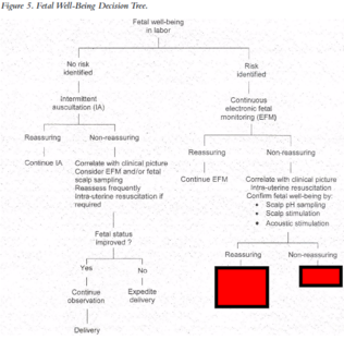
| status | not learned | measured difficulty | 37% [default] | last interval [days] | |||
|---|---|---|---|---|---|---|---|
| repetition number in this series | 0 | memorised on | scheduled repetition | ||||
| scheduled repetition interval | last repetition or drill |
Flashcard 1418210708748
| status | not learned | measured difficulty | 37% [default] | last interval [days] | |||
|---|---|---|---|---|---|---|---|
| repetition number in this series | 0 | memorised on | scheduled repetition | ||||
| scheduled repetition interval | last repetition or drill |
Open it
Meconium aspiration may cause both mechanical obstruction of the airways and chemical pneumonitis, in addition to severe pulmonary hypertension.
Flashcard 1418212281612
| status | not learned | measured difficulty | 37% [default] | last interval [days] | |||
|---|---|---|---|---|---|---|---|
| repetition number in this series | 0 | memorised on | scheduled repetition | ||||
| scheduled repetition interval | last repetition or drill |
Open it
Meconium aspiration may cause both mechanical obstruction of the airways and chemical pneumonitis, in addition to severe pulmonary hypertension.
Flashcard 1418213854476
| status | not learned | measured difficulty | 37% [default] | last interval [days] | |||
|---|---|---|---|---|---|---|---|
| repetition number in this series | 0 | memorised on | scheduled repetition | ||||
| scheduled repetition interval | last repetition or drill |
Open it
Meconium aspiration may cause both mechanical obstruction of the airways and chemical pneumonitis, in addition to severe pulmonary hypertension.
Flashcard 1418216738060
- prematurity
- abn fetus
- mult pregnancy
- polyhydramnios
- premature ROM
- AROM
- high presenting part
- obstetric procedures (ECV)
| status | not learned | measured difficulty | 37% [default] | last interval [days] | |||
|---|---|---|---|---|---|---|---|
| repetition number in this series | 0 | memorised on | scheduled repetition | ||||
| scheduled repetition interval | last repetition or drill |
Flashcard 1418218573068
| status | not learned | measured difficulty | 37% [default] | last interval [days] | |||
|---|---|---|---|---|---|---|---|
| repetition number in this series | 0 | memorised on | scheduled repetition | ||||
| scheduled repetition interval | last repetition or drill |
Open it
If infant is vigorous and crying immediately after birth, suctioning the mouth and nares is not necessarily recommended in the presence of meconium
Flashcard 1418221456652
| status | not learned | measured difficulty | 37% [default] | last interval [days] | |||
|---|---|---|---|---|---|---|---|
| repetition number in this series | 0 | memorised on | scheduled repetition | ||||
| scheduled repetition interval | last repetition or drill |
Open it
If infant is depressed at birth, tracheal intubation and suctioning of meconium from the lower airway should be done.
Flashcard 1418223029516
| status | not learned | measured difficulty | 37% [default] | last interval [days] | |||
|---|---|---|---|---|---|---|---|
| repetition number in this series | 0 | memorised on | scheduled repetition | ||||
| scheduled repetition interval | last repetition or drill |
Open it
If infant is depressed at birth, tracheal intubation and suctioning of meconium from the lower airway should be done.
Flashcard 1418225913100
| status | not learned | measured difficulty | 37% [default] | last interval [days] | |||
|---|---|---|---|---|---|---|---|
| repetition number in this series | 0 | memorised on | scheduled repetition | ||||
| scheduled repetition interval | last repetition or drill |
Flashcard 1418227748108
- check for cord pulsations
- if fetus already dead/too immature to survive/lethal anomaly, intervention for fetal reasons are inappropriate (allow vag deliv or c/s if transverse lie)
2. relieve cord compression
- if cord outside introitus, gently replace in vagina
- with hand in vagina, cradle cord in palm & use tips of fingers to elevate presenting part off of cord
- adjust maternal position to trendelenberg (head lower than pelvis) or knee-chest
3. method of delivery
- if cervix fully dilated & present part low, do assisted vag deliv
- if cervix not fully dilated/vag deliv dangerous, do immediate CS
| status | not learned | measured difficulty | 37% [default] | last interval [days] | |||
|---|---|---|---|---|---|---|---|
| repetition number in this series | 0 | memorised on | scheduled repetition | ||||
| scheduled repetition interval | last repetition or drill |
Flashcard 1418229583116
| status | not learned | measured difficulty | 37% [default] | last interval [days] | |||
|---|---|---|---|---|---|---|---|
| repetition number in this series | 0 | memorised on | scheduled repetition | ||||
| scheduled repetition interval | last repetition or drill |
|
Subject 4. Equity
#cfa #cfa-level-1 #financial-reporting-and-analysis #understanding-balance-sheets
Equity is a residual value of assets which the owner has claim to after satisfying other claims on the assets (liabilities). There are five potential components that comprise the owner's equity section of the balance sheet:
Statement of Changes in Shareholders' Equity This statement reflects information about increases or decreases to a company's net assets or wealth. It reveals much more about the year's stockholders' equity transactions than the statement of retained earnings.
|
| status | not read | reprioritisations | ||
|---|---|---|---|---|
| last reprioritisation on | suggested re-reading day | |||
| started reading on | finished reading on |
|
Subject 5. Uses and Analysis of the Balance Sheet
#cfa #cfa-level-1 #financial-reporting-and-analysis #has-images #understanding-balance-sheets
Common-Size Analysis of Balance Sheets
This topic will be discussed in detail in Reading 28 [Financial Analysis Techniques]. Balance Sheet Ratios Liquidity ratios measure the ability of a company to meet future short-term financial obligations from current assets and, more importantly, cash flows. Each of the following ratios takes a slightly different view of cash or near-cash items.
Solvency ratios measure a company's ability to meet long-term and other obligations.
Financial statement analysis aims to investigate a company's financial condition and operating performance. Using financial ratios helps to examine relationships among individual data items from financial statements. Although ratios by themselves cannot answer questions, they can help analysts ask the right questions in financial statement analysis. As analytical tools, ratios are attractive because they are simple and convenient. However, ratios are only as good as the data upon which they are based and the information with which they are compared. Fr... |


| status | not read | reprioritisations | ||
|---|---|---|---|---|
| last reprioritisation on | suggested re-reading day | |||
| started reading on | finished reading on |
|
Subject 1. Classification of Cash Flows and Non-Cash Activities
#cfa #cfa-level-1 #financial-reporting-and-analysis #understanding-cashflow-statements
The cash flow statement provides important information about a company's cash receipts and cash payments during an accounting period as well as information about a company's operating, investing and financing activities. Although the income statement provides a measure of a company's success, cash and cash flow are also vital to a company's long-term success. Information on the sources and uses of cash helps creditors, investors, and other statement users evaluate the company's liquidity, solvency, and financial flexibility.
Cash receipts and cash payments during a period are classified in the statement of cash flows into three different activities: Operating Activities These involve the cash effects of transactions that enter into the determination of net income and changes in the working capital accounts (accounts receivable, inventory, and accounts payable). Cash flows from operating activities (CFOs) reflect the company's ability to generate sufficient cash from its continuing operations. CFOs are derived by converting the income statement from an accrual basis to a cash basis. For most companies, positive operating cash flows are essential for long-run survival. The major operating cash flows are (1) cash received from customers, (2) cash paid to suppliers and employees, (3) interest and dividends received, (4) interest paid, and (5) income taxes paid. Special items to note:
Investing Activities These include making and collecting loans and acquiring and disposing of investments (both debt and equity) and property, plants, and equipment. In general, these items relate to the long-term asset items on the balance sheet. Investing cash flows reflect how a company plans its expansions. Examples are:
Financing Activities These involve liability and owner's equity items, and include:
In general, the items in this section relate to the debt and the equity items on the balance sheet. Financing cash flows reflect how the company plans to finance its expansion and reward its owners. Examples:
Purchase of debt and equity securities fro... |
| status | not read | reprioritisations | ||
|---|---|---|---|---|
| last reprioritisation on | suggested re-reading day | |||
| started reading on | finished reading on |
|
Subject 2. Preparing the Cash Flow Statement
#cfa #cfa-level-1 #financial-reporting-and-analysis #has-images #understanding-cashflow-statements
The beginning and ending cash balances on the statement of cash flows tie directly to the Cash and Cash Equivalents accounts listed on the balance sheets at the beginning and end of the accounting period.
Net income differs from net operating cash flows for several reasons.
There are two methods of converting the income statement from an accrual basis to a cash basis. Companies can use either the direct or the indirect method for reporting their operating cash flow.
Direct Method Under the direct method, the statement of cash flows reports net cash flows from operations as major classes of operating cash receipts and cash disbursements. This method converts each item on the income statement to its cash equivalent. The net cash flows from operations are determined by the difference between cash receipts and cash disbursements. Assume that Bismark Company has the following balance sheet and income statement information:

 Additional information:
Direct Method:
|
| status | not read | reprioritisations | ||
|---|---|---|---|---|
| last reprioritisation on | suggested re-reading day | |||
| started reading on | finished reading on |
|
Subject 3. Cash Flow Statement Analysis
#cfa #cfa-level-1 #financial-reporting-and-analysis #understanding-cashflow-statements
Evaluation of the Sources and Uses of Cash
Analysts should assess the sources and uses of cash between the three main categories and investigate what factors drive the change of cash flow within each category. For example, if operating cash flow is growing, does that indicate success as the result of increasing sales or expense reductions? Are working capital investments increasing or decreasing? Is the company dependent on external financing? Answers to questions like these are critical for analysts and can help form a foundation for evaluating the financial health of an industry or company. Please refer to the textbook for specific examples. Common-Size Analysis of the Statement of Cash Flows This topic will be discussed in detail in Reading 28 [Financial Analysis Techniques]. Free Cash Flow to the Firm and Free Cash Flow to Equity From an analyst's point of view, cash flows from operation activities have two major drawbacks:
Free Cash Flow (FCF) is intended to measure the cash available to a company for discretionary uses after making all required cash outlays. It accounts for capital expenditures and dividend payments, which are essential to the ongoing nature of the business. The basic definition is cash from operations less the amount of capital expenditures required to maintain the company's present productive capacity.
Free Cash Flow to the Firm (FCFF): Cash available to shareholders and bondholders after taxes, capital investment, and WC investment.
Example Quinton is evaluating Proust Company for 2014. Quinton has gathered the following information (in millions):
Calculate the FCFF for Proust for the year. Solution NCC = Depreci... |
| status | not read | reprioritisations | ||
|---|---|---|---|---|
| last reprioritisation on | suggested re-reading day | |||
| started reading on | finished reading on |
|
Subject 1. Analysis Tools and Techniques
#cfa #cfa-level-1 #financial-analysis-techniques #financial-reporting-and-analysis #has-images
Financial analysis techniques are useful in summarizing financial reporting data and evaluating the performance and financial position of companies. The results of financial techniques provide important inputs into security valuation.
Ratios Ratios express one quantity in relation to another. As analytical tools, ratios are attractive because they are simple and convenient. They can provide a profile of a company, its economic characteristics and competitive strategies, and its unique operating, financial, and investment characteristics. Ratio analysis is essential to comprehensive financial analysis. However, analysts should understand the following aspects when dealing with ratios:
Limitations: There are a significant number of estimates and subjective information that go into financial statements and therefore it is imperative that the analyst understands the numbers before calculating and relying on ratio analyses based on these numbers. An analyst needs to ask questions like:
Common-size Analysis Raw numbers hide relevant information that percentages frequently unveil. Common-size statements normalize balance sheet, income statement, and cash flow statement items to allow easier comparison of different-sized companies. They reduce all the dollar am... |
| status | not read | reprioritisations | ||
|---|---|---|---|---|
| last reprioritisation on | suggested re-reading day | |||
| started reading on | finished reading on |
|
Subject 2. Common Ratios
#cfa #cfa-level-1 #financial-analysis-techniques #financial-reporting-and-analysis #has-images
The ratios presented in the textbook are neither exclusive nor uniquely "correct." The definition of many ratios is not standardized and may vary from analyst to analyst, textbook to textbook, and annual report to annual report. The analyst's primary focus should be the relationships indicated by the ratios, not the details of their calculations.
Activity Ratios A company's operating activities require investments in both short-term (inventory and accounts receivable) and long-term (property, plant, and equipment) assets. Activity ratios describe the relationship between the company's level of operations (usually defined as sales) and the assets needed to sustain operating activities. They measure how well a company manages its various assets.
|


| status | not read | reprioritisations | ||
|---|---|---|---|---|
| last reprioritisation on | suggested re-reading day | |||
| started reading on | finished reading on |
|
Subject 3. The DuPont System
#cfa #cfa-level-1 #financial-analysis-techniques #financial-reporting-and-analysis #has-images
The breakdown of ROE into component ratios to assess the impact of those ratios is generally referred to as the DuPont Model.
Traditional DuPont equation:
Each of these components impacts the overall return to shareholders. An increase in profit margin, asset turnover, or leverage can all increase the return. There is a downside as well. If a company loses money in any year, the asset turnover or financial leverage multiplies this loss effect.
 This implies that to improve its return on equity, a company should become more:
A company's over- or underperformance on ROA is due to one or both of these causes, or "drivers." The extended DuPont model takes the above three factors and incorporates the effect of taxes and interest based on the level of financial leverage. It takes the profit margin and backs up to see the effect of interest and taxes on the overall return to shareholders. Therefore the extended model starts with EBIT (Earnings Before Interest and Taxes) rather than net income.
High financial leverage does not always increase ROE; higher financial leverage will lead to a higher interest expense rate, which may offset the benefits of higher leverage. This breakdown will help an analyst understand what happened to a company's ROE and why it happened. |
| status | not read | reprioritisations | ||
|---|---|---|---|---|
| last reprioritisation on | suggested re-reading day | |||
| started reading on | finished reading on |
|
Subject 4. Ratios Used in Equity Analysis, Credit Analysis, and Segment Analysis
#cfa #cfa-level-1 #financial-analysis-techniques #financial-reporting-and-analysis
Equity Analysis
Analysts need to evaluate a company's performance in order to value a security. One of their valuation methods is the use of valuation ratios. Some common valuations ratios are:
These price multiples and dividend-related quantities are discussed in more detail in Study Session 14 (Equity Analysis and Valuation). Credit Analysis Credit analysis is the evaluation of credit risk. How does an analyst who has calculated a ratio know whether it represents good, bad, or indifferent credit quality? Somehow, the analyst must relate the ratio to the likelihood that a borrower will satisfy all scheduled interest and principal payments in full and on time. In practice, this is accomplished by testing financial ratios as predictors of the borrower's propensity not to pay (to default). For example, a company with high financial leverage is statistically more likely to default than one with low leverage, all other factors being equal. Similarly, high fixed-charge coverage implies less default risk than low coverage. After identifying the factors that create high default risk, the analyst can use ratios to rank all borrowers on a relative scale of propensity to default. Many credit analysts conduct their ratio analyses within ranking frameworks established by their employers. In the securities field, bond ratings provide a structure for analysis. Credit rating agencies such as Moody's and Standard & Poor's use financial ratios when assigning a credit rating to a company's debt issues. For example, credit ratios used by Standard & Poor's include EBIT interest coverage, funds from operations to total debt, total debt to EBITDA, and total debt to total debt plus equity. Much research has been performed on the ability of ratios to assess the credit risk of a company (including the risk of bankruptcy) and predict bond ratings and bond yields. Segment Analysis A company may be involved in many different businesses, may do business in many different geographic areas, or may have significant number of customers. It is difficult to analyze a company with multiple business lines because of the inherent differences in financial structures, risk characteristics, etc,. amount the different lines. Aggregation of financial results for all the lines tends to obscure the true picture. A company must disclose information related to various subdivisions of its business.
|
| status | not read | reprioritisations | ||
|---|---|---|---|---|
| last reprioritisation on | suggested re-reading day | |||
| started reading on | finished reading on |
|
Subject 5. Model Building and Forecasting
#cfa #cfa-level-1 #financial-analysis-techniques #financial-reporting-and-analysis
The results of financial analysis provide valuable inputs into forecasts of future earnings and cash flow. An analyst can build a model to forecast future performance of a company. Techniques that can be used include:
|
| status | not read | reprioritisations | ||
|---|---|---|---|---|
| last reprioritisation on | suggested re-reading day | |||
| started reading on | finished reading on |
|
Subject 1. Cost of Inventories
#cfa #cfa-level-1 #financial-reporting-and-analysis #inventories #inventories-long-lived-assets-income-taxes-and-non-current-liabilities
There are two basic issues involved in inventory accounting:
1. Determine the cost of goods available for sale: Beginning Inventory + Purchases. 2. Allocate the cost of total inventory costs (cost of goods available for sale) between two components: COGS on the income statement and the ending inventory on the balance sheet. Note that COGS = (Beginning Inventory + Purchases) - Ending Inventory. The cost flow assumption to be adopted includes specific identification, average cost, FIFO, LIFO, etc. This issue will be discussed in subsequent subjects. Determination of Inventory Cost IFRS and SFAS No. 151 provide similar treatment of the determination of inventory costs. The cost of inventories, capitalized inventory costs, includes all costs incurred in bringing the inventories to their present location and condition.
|
| status | not read | reprioritisations | ||
|---|---|---|---|---|
| last reprioritisation on | suggested re-reading day | |||
| started reading on | finished reading on |
|
Subject 2. Inventory Valuation Methods
#cfa #cfa-level-1 #financial-reporting-and-analysis #inventories #inventories-long-lived-assets-income-taxes-and-non-current-liabilities
In some cases, it's possible to specifically identify which inventory items have been sold and which remain. Using the specific identification method, the actual costs of the specific units sold are transferred from inventory to the cost of goods sold. (Debit Cost of Goods Sold; Credit Inventory.) This method achieves the proper matching of sales revenue and cost of goods sold when the individual units in the inventory are unique. However, the method becomes cumbersome and may produce misleading results if the inventory consists of homogeneous items. In most cases, companies may be unable to determine exactly which items are sold and which items remain in ending inventory.
The remaining three methods are referred to as cost flow assumptions under GAAP and cost formulas under IFRS. They should be applied only to an inventory of homogeneous items. The cost flow assumption may or may not reflect the physical flow of inventory. Weighted Average Cost Using the weighted average cost method, the average cost of all units in the inventory is computed and used in recording the cost of goods sold. This is the only method in which all units are assigned the same (average) per-unit cost.
FIFO FIFO is the assumption that the first units purchased are the first units sold. Thus inventory is assumed to consist of the most recently purchased units. FIFO assigns current costs to inventory but older (and often lower) costs to the cost of goods sold. LIFO LIFO is the assumption that the most recently acquired goods are sold first. This method matches sales revenue with relatively current costs. In a period of inflation, LIFO usually results in lower reported profits and lower income taxes than the other methods. However, the oldest purchase costs are assigned to inventory, which may result in inventory becoming grossly understated in terms of current replacement costs. LIFO is not allowed under IFRS. In the U.S., however, LIFO is used by approximately 36 percent of U.S. companies because of potential income tax savings. Comparison of Inventory Accounting Methods Inventory data is useful if it reflects the current cost of replacing the inventory. COGS data is useful if it reflects the current cost of replacing the inventory items to continue operations. During periods of stable prices, all three methods will generate the same results for inventory, COGS, and earnings. During periods of rising prices and stable or growing inventories, FIFO measures assets better (the most useful inventory data) but LIFO measures income better.
In an environment of declining inventory unit costs and constant or increasing inventory quantitie... |
| status | not read | reprioritisations | ||
|---|---|---|---|---|
| last reprioritisation on | suggested re-reading day | |||
| started reading on | finished reading on |
|
Subject 3. Periodic versus Perpetual Inventory System
#cfa #cfa-level-1 #financial-reporting-and-analysis #inventories #inventories-long-lived-assets-income-taxes-and-non-current-liabilities
The perpetual inventory system updates inventory accounts after each purchase or sale. Inventory quantities are updated continuously. When there is a sale, inventory is reduced and COGS is calculated.
The periodic inventory system records inventory purchase or sale in the "Purchases" account. The "Inventory" account is updated on a periodic basis, at the end of each accounting period (e.g., monthly, quarterly). Cost of goods sold or cost of sale is computed from the ending inventory figure. With perpetual FIFO, the first (or oldest) costs are the first moved from the Inventory account and debited to the Cost of Goods Sold account. The end result under perpetual FIFO is the same as under periodic FIFO. In other words, the first costs are the same whether you move the cost out of inventory with each sale (perpetual) or whether you wait until the year is over (periodic). With perpetual LIFO, the last costs available at the time of the sale are the first to be removed from the Inventory account and debited to the Cost of Goods Sold account. Since this is the perpetual system, we cannot wait until the end of the year to determine the last cost. An entry must be recorded at the time of the sale in order to reduce the Inventory account and increase the Cost of Goods Sold account. If costs continue to rise throughout the entire year, perpetual LIFO will yield a lower cost of goods sold and a higher net income than periodic LIFO. Generally this means that periodic LIFO will result in lower income taxes than perpetual LIFO. Example Date....................................Units....Price 12.31.2008........Beginning Inventory....1.......85 1.1.2009..........Purchase...............1.......87 2.1.2009..........Purchase...............2.......89 6.1.2009..........Sales..................1.......89 12.1.2009.........Purchase...............1.......90 Under perpetual LIFO the following entry must be made at the time of the sale: $89 will be credited to Inventory and $89 will be debited from Cost of Goods Sold. If that was the only item sold during the year, at the end of the year the Cost of Goods Sold account will have a balance of $89 and the cost in the Inventory account will be $351 ($85 + $87 + $89 + $90). Under periodic LIFO we assign the last cost of $90 to the one item that was sold. (If two items were sold, $90 would be assigned to the first item and $89 to the second item.) The remaining $350 is assigned to inventory. The $350 of inventory cost consists of $85 + $87 + $89 + $89. The $90 assigned to the item that was sold is permanently gone from inventory. |
| status | not read | reprioritisations | ||
|---|---|---|---|---|
| last reprioritisation on | suggested re-reading day | |||
| started reading on | finished reading on |
|
Subject 4. The LIFO Method
#cfa #cfa-level-1 #financial-reporting-and-analysis #inventories #inventories-long-lived-assets-income-taxes-and-non-current-liabilities
In the U.S., firms that use LIFO must report a LIFO reserve. The LIFO reserve is the difference between the inventory balance shown on the balance sheet and the amount that would have been reported had the firm used FIFO. That is:
It represents the cumulative effect over time of ending inventory under LIFO vs. FIFO. When adjusting COGS from LIFO to FIFO: COGSFIFO = COGSLIFO - Change in LIFO Reserve. LIFO Liquidations So far, discussions have been based on the assumptions of rising prices and stable or growing inventory quantity. As a result, the LIFO reserve increases over time. However, LIFO reserves can decline for either of the two reasons listed below. In either case, the COGS will be smaller and the reported income will be higher relative to what they would have been if the LIFO reserve had not declined. However, the implications of a decline in the LIFO reserve on financial analysis vary, depending on the reason for the decline.
|
| status | not read | reprioritisations | ||
|---|---|---|---|---|
| last reprioritisation on | suggested re-reading day | |||
| started reading on | finished reading on |
|
Subject 5. Measurement of Inventory Value
#cfa #cfa-level-1 #financial-reporting-and-analysis #inventories #inventories-long-lived-assets-income-taxes-and-non-current-liabilities
Under IFRS, inventories are reported at the lower of cost or net realizable value (NRV).
IFRS does not apply to the measurement of inventories held by producers of agricultural and forest products, mineral products, or commodity brokers and dealers. Their inventories are measured at net realizable value (above or below cost) in accordance with well-established practices in those industries. Similarly, GAAP requires the use of the lower-of-cost-or-market valuation basis (LCM) for inventories, with market value defined as replacement cost. Reversal is prohibited, however. The LCM valuation basis follows the principle of conservatism (on both the balance sheet and income statement) since it recognizes losses or declines in market value as they occur, whereas increases are reported only when inventory is sold. Here are some relevant terms:
Example Historical cost: $5,000 Market cost: $2,000 Estimated selling price: $4,000 Estimated costs to complete sale: $1,000 Net realizable value: $4,000 - $1,000 = $3,000
Now assume NRV increases from $3,000 to $4,000 and the market cost increases from $2,000 to $3,000.
|
| status | not read | reprioritisations | ||
|---|---|---|---|---|
| last reprioritisation on | suggested re-reading day | |||
| started reading on | finished reading on |
|
Subject 6. Financial Analysis of Inventories
#cfa #cfa-level-1 #financial-reporting-and-analysis #has-images #inventories #inventories-long-lived-assets-income-taxes-and-non-current-liabilities
Financial statement disclosures provide information regarding the accounting policies adopted in measuring inventories, the principal uncertainties regarding the use of estimates related to inventories, and details of the inventory carrying amounts and costs. This information can greatly assist analysts in their evaluation of a company's inventory management.
Presentation and Disclosure Consistency of inventory accounting policy is required under both U.S. GAAP and IFRS. If a company changes an inventory accounting policy, the change must be justifiable and all financial statements accounted for retrospectively. The one exception is for a change to the LIFO method under U.S. GAAP; the change is accounted for prospectively and there is no retrospective adjustment to the financial statements. Inventory Ratios Inventory turnover measures how fast a company moves its inventory through the system.
 This ratio can be used to measure how well a firm manages its inventories. The lower the ratio, the longer the time between when the good is produced or purchased and when it is sold.
 Financial Analysis: FIFO versus LIFO The advantages of LIFO are:
The disadvantages of LIFO:
|
| status | not read | reprioritisations | ||
|---|---|---|---|---|
| last reprioritisation on | suggested re-reading day | |||
| started reading on | finished reading on |
|
Subject 1. Capitalizing versus Expensing
#cfa #cfa-level-1 #financial-reporting-and-analysis #inventories-long-lived-assets-income-taxes-and-non-current-liabilities #long-lived-assets
The costs of acquiring resources that provide services over more than one operating cycle should be capitalized and carried as assets on the balance sheet. All costs incurred until an asset is ready for use must be capitalized, including the invoice price, applicable sales tax, freight and insurance costs incurred delivering equipment, and any installation costs. Costs of the long-lived asset should be allocated over current and future periods. In contrast, if these assets are expensed, their entire costs are written off as expense on the income statement in the current period. Accounting rules on capitalization are not straightforward. As a result, management has considerable discretion in making decisions such as whether to capitalize or expense the cost of an asset, whether to include interest costs incurred during construction in the capitalized cost, and what types of costs to capitalize for intangible assets. The choice of capitalization or expensing affects the balance sheet, income and cash flow statements, and ratios both in the year the choice is made and over the life of the asset. Here is a summary of the different effects of capitalization versus expensing:
Under SFAS 34, interest is capitalized for certain assets and only if the firm is leveraged. Therefore, the carrying amount of a self-constructed asset depends on the firm's financial decisions. The capitalized interest cost is added to the value of the asset being constructed. The amount of interest cost to be capitalized has two components:
Therefore, the total interest cost incurred during the accounting period has two parts:
The total interest cost, along with the amount capitalized, must be disclosed as part of the notes to the financial statements. Once the construction is complete, capitalized interest costs will be written off as part of depreciation over the useful life of the asset. From ... |
| status | not read | reprioritisations | ||
|---|---|---|---|---|
| last reprioritisation on | suggested re-reading day | |||
| started reading on | finished reading on |
|
Subject 2. Intangible Assets
#cfa #cfa-level-1 #financial-reporting-and-analysis #inventories-long-lived-assets-income-taxes-and-non-current-liabilities #long-lived-assets
Intangible assets are identifiable nonmonetary resources controlled by firms. Examples include patents, copyrights, franchises, goodwill, trademarks, trade names, secret processes, property rights, and organization costs.
Accounting for the Acquisition of Long-Lived Intangible Assets Accounting for an intangible asset depends on how it is acquired. 1. Intangible Assets Purchased in Situations Other than Business Combinations These are accounted for at acquisition costs. "Cost" includes purchase price, legal fees, and other expenses that make the intangibles ready for use. For example, fees paid to obtain a license or franchise are capitalized. Another example: expenditures on patents and copyrights purchased from another party are capitalized. They are amortized over their remaining legal lives or 40 years, whichever is less. The straight-line method is typically used for amortization. 2. Intangible Assets Developed Internally For internally generated intangible assets, it is difficult to measure costs, benefits, and economic lives. Generally, internally generated assets (such as costs of R&D, patents and copyrights, brands and trademarks, and advertising and secret processes) must be expensed in the period incurred. One exception is research and development (R&D) expenditures which add risk to investment with uncertain future economic benefits. As a result, they must be expensed as incurred in most countries (including the U.S.). SFAS 86 requires that all R&D costs to establish the technological and/or economic feasibility of software must be expensed. Subsequent costs that are beyond the point of technological feasibility can - but don't have to - be capitalized as part of product inventory and amortized based on revenues or on a straight-line basis. The point of technological feasibility is the point when a software prototype has been proven to be technologically feasible, as evidenced by the existence of a working model of the software. IFRS also requires research costs be expensed but allows development costs to be capitalized under certain conditions. As you can see, managers have considerable discretion in making decisions, such as whether or when to capitalize these costs and by how much. For software development costs, one particular risk is that capitalized costs will not be realized and a future write-down may be needed. If companies apply different approaches to capitalizing software development costs, adjustments can be made to make the two comparable. 3. Intangible Assets Acquired in a Business Combination Business combinations are accomplished when one entity (investor) acquires "control" over the net assets of another entity. The transaction is accounted for using the purchase method of accounting, in which the company identified as the acquirer allocates the purchase price to each asset acquired (and each liability assumed) on the basis of its fair value. Any excess of cost over fair value of net assets acquired is recorded as goodwill. U.S. GAAP requires that in-process R&D (IPRD) of the target company should be expensed at the date of acquisition, which results in a large one-time charge. IFRS requires identifying IFRD as a separate asset with a finite life or including it as part of goodwill. Amortizing Intangible Assets with Finite Useful Lives An intangible asset with a finite useful life is amortized over its useful life. The estimates required for amortization calculations are: original valuation amount, residual value at the end of useful life, and the length of useful life. Example Torch, Inc. has developed a new device. Patent registration costs consisted of $2,000 in attorney fees and $1,000 in federal registration fees. The device has a useful life of 5 years. The legal life is 17 y... |
| status | not read | reprioritisations | ||
|---|---|---|---|---|
| last reprioritisation on | suggested re-reading day | |||
| started reading on | finished reading on |
|
Subject 3. Depreciation Methods
#cfa #cfa-level-1 #financial-reporting-and-analysis #has-images #inventories-long-lived-assets-income-taxes-and-non-current-liabilities #long-lived-assets
For accountants, depreciation is an allocation process, not a valuation process. It is important for analysts to differentiate between accounting depreciation and economic depreciation. Two factors affect the computation of depreciation: depreciable cost (acquisition cost - salvage or residual value) and estimated useful life (depreciable life). Note that it is depreciable cost, not acquisition cost, that is allocated over the useful life of an asset.
The different depreciation methods are:
|


| status | not read | reprioritisations | ||
|---|---|---|---|---|
| last reprioritisation on | suggested re-reading day | |||
| started reading on | finished reading on |
|
Subject 4. The Revaluation Model
#cfa #cfa-level-1 #financial-reporting-and-analysis #inventories-long-lived-assets-income-taxes-and-non-current-liabilities #long-lived-assets
Under U.S. accounting standards, it is compulsory to account for impairment in long-lived assets (downward revaluation). However, upward revaluation of long-lived assets to reflect fair market values is not allowed.
The balance sheet is more informative when assets and liabilities are stated at market value rather than historical cost. IASB and some other non-U.S. GAAP do permit upward revaluations. The purpose of a revaluation is to bring into the books the fair market value of long-lived assets.
Financial Statement Analysis Considerations
|
| status | not read | reprioritisations | ||
|---|---|---|---|---|
| last reprioritisation on | suggested re-reading day | |||
| started reading on | finished reading on |
|
Subject 5. Impairment of Assets
#cfa #cfa-level-1 #financial-reporting-and-analysis #inventories-long-lived-assets-income-taxes-and-non-current-liabilities #long-lived-assets
Sometimes a long-term asset may lose some of its revenue-generating ability prior to the end of its useful life. (e.g., a significant decrease in the market value, physical change, or use of the assets). If the carrying amount of the asset is determined not to be recoverable, an asset impairment occurs and the carrying value should be written down. The amount of the write-down is recorded as a loss.
GAAP and IFRS differ as to the methodology used to determine impairment. The GAAP methodology of determining impairment uses a two-step recoverability test. Occurrence of an impairment differs from recognition of an impairment. An impairment, whether recognized in financial reports or not, occurs as long as an asset's carrying value cannot be fully recovered in the future. However, only impairments that meet certain conditions are recognized in financial reports. SFAS 121 provides a two-step process:
Conversely, IFRS methodology uses a one-step approach. This approach requires that impairment loss be calculated if "impairment indicators" exist. This approach does not rely on net undiscounted future cash flows and subsequent comparison to asset carrying value as required in GAAP methodology. In addition, the impairment loss is calculated as the amount by which the carrying amount of the asset exceeds it recoverable amount. The recoverable amount is the higher of the following: 1) fair value less cost to sell, or 2) value in use (i.e., the present value of future cash flows including disposal value). Impairment of Intangible Assets
Among the most interesting intangible assets is goodwill. Goodwill is the present value of future earnings in excess of a normal return on net identifiable assets. It stems from such factors as a good reputation, loyal customers, and superior management. Any business that earns significantly more than a normal rate of return actually has goodwill. Goodwill is recorded in the accounts only if it is purchased by acquiring another business at a price higher than the fair market value of its net identifiable assets. It is not valued directly but inferred from the values of the acquired assets compared with the purchase price. It is the premium paid for the target company's reputation, brand names, customers or suppliers, technical knowledge, key personnel, and so forth. Goodwill only has value insofar as it represents a sustainable competitive advantage that will result in abnormally high earnings. Analysts need to be aware of the possibility that the goodwill recognized by accountants may, in fact, represent overpayment for the acquired company. Since goodwill is inferred rather than computed directly, it will increase as the payment price increases. It is only after the passage of time that analysts will be able to evaluate the extent to which the purchase price was justified. Under U.S. GAAP SFAS 142, goodwill is not amortized, but is tested annually for impairment. Goodwill impairment for each reporting unit should be tested in a two-step process at least once a year. 1. The fair value of a reporting unit is compared to its ... |
| status | not read | reprioritisations | ||
|---|---|---|---|---|
| last reprioritisation on | suggested re-reading day | |||
| started reading on | finished reading on |
|
Subject 6. Derecognition
#cfa #cfa-level-1 #financial-reporting-and-analysis #has-images #inventories-long-lived-assets-income-taxes-and-non-current-liabilities #long-lived-assets
For accounting purposes, an asset may be disposed of in three different ways. It may be:
When plant assets are disposed of, depreciation should be recorded on the date of disposal. The cost is then removed from the asset account and the total recorded depreciation is removed from the accumulated depreciation account. Normally an asset's market value at the time of sale or disposal will most likely be different than the asset's book value (its original historical cost minus all accumulated depreciation on that asset). The sale of a plant asset at a price above or below book value results in a gain or loss to be reported in the income statement. Because different depreciation methods are used for income tax purposes, the gain or loss reported on income tax returns may differ from that shown in the income statement. It is the gain or loss shown in the financial statement that is recorded in the company's general ledger accounts. To illustrate each of these methods consider this. A machine was purchased on 1 January Year 1 for $1,000. The depreciation method was straight-line with a useful-life of 5 years and an estimated residual value of $200. On 31 July Year 3 the firm decides to dispose of the asset. The firm has a December year-end. The first step irrespective of the method of disposal is to calculate the depreciation up to the date of sale: Depreciation per year = (Cost - residual value) / Useful life = (1,000 - 200) / 5 = $160 Depreciation for year 1 = $160 Depreciation for year 2 = $160 Depreciation for year 3 = $93 (160 x 7/12) Total: $413 Remember that the depreciation for year 3 is only for 7 months, as the asset is disposed of on 31 July Year 3. Sale of Long-Lived Assets The gain or loss on the sale of long-lived assets is computed as the sales proceeds minus the carrying value of the asset at the time of sale. Assume that the machinery is sold for cash in three scenarios: a. Sold for $587 cash (Sale of machinery for carrying value) Debit: Cash (B/S) $587 Debit: Accumulated depreciation (B/S) $413 Credit: Machinery (B/S) $1000 b. Sold for $600 cash (Sale of machinery for above carrying value) Debit: Cash (B/S) $600 Debit: Accumulated depreciation (B/S) $413 Credit: Machinery (B/S) $1000 Credit: Profit on sale of machinery (I/S) $13 c. Sold for $500 cash (Sale of machinery for below carrying value) Debit: Cash (B/S) $500 Debit: Accumulated depreciation (B/S) $413 Debit: Loss on sale of machinery (I/S) $87 Credit: Machinery (B/S) $1000 In summary, when disposing of an asset, entries are prepared to:
Exchange of Long-Lived Assets If an asset is exchanged for another asset, the basic accounting is similar to the accounting for sales of plant assets for cash. If the trade-in allowance received is greater than the carrying value of the asset surrendered, there has been a gain. If the allowance is less, there has been a loss. Level II will cover some special rules for recognizing these gains and losses, depending on the nature of the assets exchanged:
 Abandoned If an a... |
| status | not read | reprioritisations | ||
|---|---|---|---|---|
| last reprioritisation on | suggested re-reading day | |||
| started reading on | finished reading on |
|
Subject 7. Presentation and Disclosures
#cfa #cfa-level-1 #financial-reporting-and-analysis #inventories-long-lived-assets-income-taxes-and-non-current-liabilities #long-lived-assets
Property, Plant, and Equipment (PP&E)
IAS 16 provides a long list of disclosure requirements for PP&E. For each class of PP&E, the financial statements must disclose the following:
U.S. GAAP require a company to disclose the depreciation expense for the period, the balances of assets, accumulated depreciation and a general description of the depreciation method(s) used. Intangible Assets IAS 38 provides a considerable set of disclosure requirements for intangible assets. For each class of intangibles, and distinguishing between internally generated and other assets, the financial statements must disclose:
Under U.S. GAAP, a company is required to disclose the gross carrying amounts and accumulated amortization, the aggregated amortization expense for the period, and the estimated amortization expense for the next 5 years. Impairment of Assets As with most other standards, IAS 36 provides a long list of disclosure requirements. To begin with, for each class of assets, the financial statements must disclose:
U.S. GAAP require a company to disclose a description of the impaired asset, what caused impairment, the method of determining fair value, the amount of impairment loss, and where the loss is recognized on the financial statements. |
| status | not read | reprioritisations | ||
|---|---|---|---|---|
| last reprioritisation on | suggested re-reading day | |||
| started reading on | finished reading on |
|
Subject 8. Investment Property
#cfa #cfa-level-1 #financial-reporting-and-analysis #inventories-long-lived-assets-income-taxes-and-non-current-liabilities #long-lived-assets
Investment property is defined as property that is owned (or, in some cases, leased under a finance lease) for the purpose of earning rental income, capital appreciation, or both.
Under IFRS, companies are allowed to value investment properties using either a cost model or a fair value model.
Under U.S. GAAP, there is no specific definition of investment property. Investment properties are generally measured using the cost model. |
| status | not read | reprioritisations | ||
|---|---|---|---|---|
| last reprioritisation on | suggested re-reading day | |||
| started reading on | finished reading on |
|
Subject 1. Key Terms
#cfa #cfa-level-1 #financial-reporting-and-analysis #income-taxes #inventories-long-lived-assets-income-taxes-and-non-current-liabilities
The computation of income taxes poses problems in financial reporting. The major problems arise because current period taxable income is measured using different rules than those used in accounting for pretax income.
Taxes are paid based on tax reporting, but from a financial reporting standpoint, the tax expense in the income statement (IS) is based on the matching principle and is computed on pretax accounting income. In order to achieve matching between taxes based on taxable income and taxes based on pretax income for accounting purposes, deferred tax entries are put through the accounting books. The differences between the tax expense for tax and the accounting tax expense create deferred tax liabilities (credits) and deferred tax assets (debits or prepaid taxes). Here are key terms based on tax return:
Here are key terms based on financial reporting:
|
| status | not read | reprioritisations | ||
|---|---|---|---|---|
| last reprioritisation on | suggested re-reading day | |||
| started reading on | finished reading on |
|
Subject 2. Deferred Tax Assets and Liabilities
#cfa #cfa-level-1 #financial-reporting-and-analysis #has-images #income-taxes #inventories-long-lived-assets-income-taxes-and-non-current-liabilities
Tax reporting and financial reporting are based on two different sets of assumptions. This is particularly true in the U.S. because financial reporting does not have to conform to tax reporting, as it does in Japan, Germany, and Switzerland. Numerous items create differences between accounting profit and taxable income. As a result, the taxes payable for the period are often different from the tax expenses recognized in the financial statements.
In the U.S.:
Because of the differences between tax accounting and financial accounting, the financial statements may include tax liabilities or assets - allowances that have been made in the financial statements for taxes that have not yet been or have already been paid. Deferred tax liabilities generally arise when tax relief is provided in advance of an accounting expense, or when income is accrued but not taxed until received. Deferred tax liabilities on an individual transaction are expected to be reversed when these liabilities are settled, causing future cash outflows. A typical example is depreciation: a company uses the Accelerated Cost Recovery System for tax reporting but uses straight-line depreciation for financial reporting.
Deferred tax assets generally arise when tax relief is provided after an expense is deducted for accounting purposes. Deferred tax assets on an individual transaction are expected to be reversed when these assets are recovered, causing future cash inflows. Different treatments of warranty expenses in tax reporting and financial reporting are a common cause of deferred tax assets:
In the U.S., deferred tax assets/liabilities are classified on the balance sheet as current or non-current based on the classification of the underlying asset or liability. However, deferred tax assets/liabilities are always classified as non-current under IFRS. A deferred tax item cannot be created if it is doubtful that the company will realize economic benefits in the future. Example A company purchases an asset for $1,000 at the beginning of Year 1. It depreciates the asset at 33% per annum (straight-line) for financial reporting. The tax depreciation is 50% per annum (straight-line). The pretax income and taxable income are $2,0... |
| status | not read | reprioritisations | ||
|---|---|---|---|---|
| last reprioritisation on | suggested re-reading day | |||
| started reading on | finished reading on |
|
Subject 3. Determining the Tax Base of Assets and Liabilities
#cfa #cfa-level-1 #financial-reporting-and-analysis #income-taxes #inventories-long-lived-assets-income-taxes-and-non-current-liabilities
The tax base of an asset or liability is the amount attributed to that asset or liability for tax purposes.
The Tax Base of an Asset An asset's tax base is the amount that will be deductible for tax purposes against any taxable economic benefits that will flow to an entity when it recovers the asset's carrying amount. It is the amount that would be tax deductible if the asset was sold on the balance sheet date. For example, a firm has total accounts receivable of $100,000. At the end of the year, management recognized a specific doubtful debt division of $3,000 for financial reporting. However, provisions for doubtful debts are not allowed for tax purposes in the firm's tax jurisdiction. A tax deduction is received when the receivable is written off as bad debt. The carrying amount of the accounts receivable becomes $97,000. The tax base of the asset still remains $100,000. The firm has a deductible temporary difference of $3,000. Management should recognize a deferred tax asset in respect to the deductible temporary difference. If the economic benefit will not be taxable, the tax base of the asset will be equal to the carrying amount of the asset. An example is dividends receivable from a subsidiary. If it is not taxable, the tax base and the carrying amount of the dividends receivable are equal. The Tax Base of a Liability The tax base of a liability is its carrying amount, less any amount that will be deductible for tax purposes with respect to that liability in future periods.
Example At the beginning of the year a firm received a lump sum of $5 million for rent from a lessee. The rent was for the use of an office building for the next 5 years. Local tax authorities require 70% of rent received in advance to be taxable income. At the end of the year, $4 million should be treated as a liability for financial reporting purposes. That's the carrying amount. The tax base of the liability is $1.2 million (30% of $4 million) and $2.8 million should be treated as taxable income. Changes in Income Tax Rates When tax rates change, the deferred tax liability or asset has to be adjusted immediately to the new amount that is now expected, based upon the new expected tax consequences. The effect of this change in estimate will be included in the income from continuing operations. The effect of an income tax rate increase:
|
| status | not read | reprioritisations | ||
|---|---|---|---|---|
| last reprioritisation on | suggested re-reading day | |||
| started reading on | finished reading on |
|
Subject 4. Temporary versus Permanent Differences
#cfa #cfa-level-1 #financial-reporting-and-analysis #has-images #income-taxes #inventories-long-lived-assets-income-taxes-and-non-current-liabilities
Numerous items create differences between accounting profit and taxable income. These differences can be divided into two types.
Permanent differences do not cause deferred tax liabilities or assets. These occur if a revenue or expense item:
Therefore, permanent differences result from revenues and expenses that are reportable on either tax returns or in financial statements but not both. Permanent differences arise because the tax code excludes certain revenues from taxation and limits the deductibility of certain expenses.
These differences are permanent because they will not reverse in future periods. No deferred tax consequences are recognized for permanent differences; however, they result in a difference between the effective tax rate and the statutory tax rate that should be considered in the analysis of effective tax rates. Example A company owns a $50,000 municipal bond with a 4% coupon and has an effective tax rate of 50% and a statutory tax rate of 40%. Calculate the deferred tax created by this bond. Solution The bond does not result in deferred tax, as the difference it causes is a permanent difference that will not reverse. As a result, no deferred tax is recognized. Temporary differences result in deferred tax liabilities or assets. Different depreciation methods or estimates used in tax reporting and financial reporting are a common cause of temporary differences. There are two categories of temporary differences. Taxable Temporary Differences (TTD)
Items that give rise to taxable temporary differences are:
Deductible Temporary Differences (DTD)
Items that give rise to deductible temporary differences are:
 |
| status | not read | reprioritisations | ||
|---|---|---|---|---|
| last reprioritisation on | suggested re-reading day | |||
| started reading on | finished reading on |
Flashcard 1418357247244
| status | not learned | measured difficulty | 37% [default] | last interval [days] | |||
|---|---|---|---|---|---|---|---|
| repetition number in this series | 0 | memorised on | scheduled repetition | ||||
| scheduled repetition interval | last repetition or drill |
|
Subject 5. Recognition and Measurement of Current and Deferred Tax
#cfa #cfa-level-1 #financial-reporting-and-analysis #income-taxes #inventories-long-lived-assets-income-taxes-and-non-current-liabilities
Deferred tax assets and liabilities are re-assessed on each balance sheet date.
Valuation Allowance Deferred tax assets are reduced by a valuation allowance to amounts that are "more likely than not" to be realized, taking into account all available positive and negative evidence about the future. For determining whether deferred tax assets must be reduced by a valuation allowance, all available positive and negative evidence must be considered. Information concerning recent pretax accounting earnings generally is critical. For example, if a firm has been recording material cumulative losses recently, it will be hard to justify a conclusion that tax credits can be realized in the near future. This will be evidence supporting the use of a valuation allowance ("negative evidence"). It is not necessary to quantify positive evidence for the conclusion that a valuation allowance is not required unless significant negative evidence exists. Where both positive and negative evidence exist, judgment must be used in evaluating what evidence is more persuasive. More weight should be given to objectively verifiable evidence. Recognition of Current and Deferred Tax Charged Directly to Equity A firm's deferred tax liability during an accounting period represents the portion of income tax expense that has not been paid. Therefore, from a pure accounting perspective, deferred tax liabilities are an accounting liability. However, from a financial analyst's perspective, whether deferred tax liabilities should be considered liabilities or not depends on whether they will reverse in the future. If they will, resulting in a cash outflow, then they should be treated as liabilities. If not, then they should be treated as equity! As deferred tax liabilities are created by temporary differences, reversal of a deferred tax liability depends on the reversal of the temporary difference that created it. Changes in a firm's operations or tax law may result in deferred taxes that are never paid or recovered. For example, the use of accelerated depreciation methods for tax reporting creates a temporary difference. Normally, when there is less depreciation in later years, the deferred tax liability created by more depreciation in earlier years will be reversed. However, for firms with high growth rates, increased investments in fixed assets result in ever-increasing new deferred tax liabilities, which replace the reversing one. That is, a firm's growth may continually generate deferred tax liabilities. In this case, the deferred taxes are unlikely to be paid. Therefore, for such high-growth firms, deferred tax liabilities will not reverse and should be treated as equity. Deferred tax liabilities are recorded at their stated value. Even if deferred taxes are eventually paid, payments typically occur far in the future. The present value of those payments is considerably lower than the stated amounts. Thus, the deferred tax liability should be discounted at an appropriate interest rate and the difference should be treated as equity. In some cases, financial statement depreciation understates the value of economic depreciation. Instead, the accelerated depreciation in tax reporting is a better measure. Examples of such cases include equipment obsolescence due to technology innovation and rising price levels. Deferred tax liabilities are neither liabilities nor equity if they are not expected to reverse, and should be ignored by financial analysts.
|
| status | not read | reprioritisations | ||
|---|---|---|---|---|
| last reprioritisation on | suggested re-reading day | |||
| started reading on | finished reading on |
Flashcard 1418359606540
| status | not learned | measured difficulty | 37% [default] | last interval [days] | |||
|---|---|---|---|---|---|---|---|
| repetition number in this series | 0 | memorised on | scheduled repetition | ||||
| scheduled repetition interval | last repetition or drill |
Flashcard 1418362752268
| status | not learned | measured difficulty | 37% [default] | last interval [days] | |||
|---|---|---|---|---|---|---|---|
| repetition number in this series | 0 | memorised on | scheduled repetition | ||||
| scheduled repetition interval | last repetition or drill |
|
Subject 7. Comparison of IFRS and U.S. GAAP
#cfa #cfa-level-1 #financial-reporting-and-analysis #income-taxes #inventories-long-lived-assets-income-taxes-and-non-current-liabilities
Similarities
FAS 109 Accounting for Income Taxes and IAS 12 Income Taxes provide the guidance for income tax accounting under U.S. GAAP and IFRS, respectively. Both pronouncements require entities to account for both current tax effects and expected future tax consequences of events that have been recognized (that is, deferred taxes) using an asset and liability approach. Further, deferred taxes for temporary differences arising from non-deductible goodwill are not recorded under either approach and the tax effects of items directly accounted for as equity during the current year are also allocated directly to equity. Finally, neither principle permits the discounting of deferred taxes. Significant Differences and Convergence Below we discuss the significant differences in the current literature. Tax basis:
Uncertain tax positions:
Initial recognition exemption:
Recognition of deferred tax assets:
Calculation of deferred asset or liability:
Classification of deferred tax assets and liabilities in balance sheet:
Recognition of deferred tax liabilities from investments in subsidiaries or joint ventures (JVs) (often referred to as outside basis differences):
|
| status | not read | reprioritisations | ||
|---|---|---|---|---|
| last reprioritisation on | suggested re-reading day | |||
| started reading on | finished reading on |
|
Subject 1. Reporting Quality and Results Quality
#cfa #cfa-level-1 #financial-reporting-and-analysis #financial-reporting-quality
Financial reporting quality: a subjective evaluation of the extent to which financial reporting is free of manipulation and accurately reflects the financial condition and operating success of a company. It pertains to the information disclosed. Earnings are considered to be high quality if they exhibit persistence and are unbiased. Sustainable earnings enable better forecasts of future cash flows or earnings. This is referred to as results quality or earnings quality. Financial reporting quality is different from earnings quality. The two concepts are, however, interrelated because a correct assessment of earnings quality is possible only if we have some basic level of financial reporting quality. Low financial reporting quality makes it hard to assess earnings quality. |
| status | not read | reprioritisations | ||
|---|---|---|---|---|
| last reprioritisation on | suggested re-reading day | |||
| started reading on | finished reading on |
|
Subject 2. Quality Spectrum of Financial Reports
#cfa #cfa-level-1 #financial-reporting-and-analysis #financial-reporting-quality
Financial reporting quality varies across companies.
GAAP, Decision-Useful, Sustainable, and Adequate Returns
GAAP, Decision-Useful, but Sustainable?
Biased Accounting Choices
Departures from GAAP It is difficult or impossible to assess earnings quality. Engaging in fraudulent financial reporting provides no quality of earnings. Conservative and Aggressive Accounting An aspect of financial reporting quality is the degree to which accounting choices are conservative or aggressive. "Aggressive" typically refers to choices that aim to enhance a company's reported performance and financial position by inflating the amount of revenues, earnings, and/or operating cash flow reported in the period or by decreasing the amount of expenses reported in the period and/or the amount of debt reported on the balance sheet. Conservatism in financial reports can result from either (1) accounting standards that specifically require a conservative treatment of a transaction or an event or (2) judgments necessarily made by managers when applying accounting standards that result in more or less conservative results. An example of conservatism in the oil and gas industry is the revenue recognition accounting standard. This standard permits recognition of revenue only at the time of shipment rather than closer to the time of actual value creation (which is the time of discovery). Big Bath Accounting The strategy of manipulating a company's income statement to make poor results look even worse. The big bath is often implemented in a bad year to artificially enhance next year's earnings. The big rise in earnings might result in a larger bonus for executives. Cookie Jar Reserve Accounting Companies shift earnings around by creating overly large reserve accounts in good years then drawing them down in bad years. |
| status | not read | reprioritisations | ||
|---|---|---|---|---|
| last reprioritisation on | suggested re-reading day | |||
| started reading on | finished reading on |
|
Subject 3. Context for Assessing Financial Reporting Quality
#cfa #cfa-level-1 #financial-reporting-and-analysis #financial-reporting-quality
Motivations for managers to issue less than high quality financial reports:
Management might have an incentive to manipulate earnings lower as well, possibly to smooth higher earnings in the current quarter into weaker quarters. Conditions conductive to issuing low-quality financial reports:
Mechanisms that discipline financial reporting quality:
|
| status | not read | reprioritisations | ||
|---|---|---|---|---|
| last reprioritisation on | suggested re-reading day | |||
| started reading on | finished reading on |
Flashcard 1418373762316
- 1/3 will stay as is
- 1/3 will progress
| status | not learned | measured difficulty | 37% [default] | last interval [days] | |||
|---|---|---|---|---|---|---|---|
| repetition number in this series | 0 | memorised on | scheduled repetition | ||||
| scheduled repetition interval | last repetition or drill |
|
Subject 4. Detection of Financial Reporting Quality Issues
#cfa #cfa-level-1 #financial-reporting-and-analysis #financial-reporting-quality
There is really nothing new in this reading, just a review of the previous material. A lot of the accounting practices are highlighted elsewhere in the curriculum but are reiterated here.
Presentation Choice If a company uses a non-GAAP financial measure in an SEC filing, it is required to provide the most directly comparable GAAP measure with equivalent prominence in the filing. In addition, the company is required to provide a reconciliation between the non-GAAP measure and the equivalent GAAP measure. Similarly, IFRS require that any non-IFRS measures included in financial reports must be defined and their potential relevance explained. The non-IFRS measures must be reconciled with IFRS measures. Accounting Choices and Estimates Managers' considerable flexibility in choosing their companies' accounting policies and formulating estimates provides opportunities for aggressive accounting. Examples include:
Cash flow, especially operating cash flow and free cash flow, are always at the heart of any discussion of financial performance and valuation. Investors, creditors, and analysts are all interested in whether a firm is generating cash flow and where that cash flow can be expected to recur. Operating cash flow is usually unaffected by estimates and judgments. However, firms can still create the perception that sustainable operating cash flow is greater than it actually is. One technique is to misrepresent a firm's cash-generating ability by classifying financing activities as operating activities and vice versa. Additionally, management has discretion over the timing of cash flows and where to report cash flows. Warning Signs Analysts should pay attention to:
|
| status | not read | reprioritisations | ||
|---|---|---|---|---|
| last reprioritisation on | suggested re-reading day | |||
| started reading on | finished reading on |
Flashcard 1418376121612
| status | not learned | measured difficulty | 37% [default] | last interval [days] | |||
|---|---|---|---|---|---|---|---|
| repetition number in this series | 0 | memorised on | scheduled repetition | ||||
| scheduled repetition interval | last repetition or drill |
Open it
evasion of host immune system + integration of HPV DNA into susceptible epithelial cells in transformation zone → cervical cancer
Flashcard 1418377694476
| status | not learned | measured difficulty | 37% [default] | last interval [days] | |||
|---|---|---|---|---|---|---|---|
| repetition number in this series | 0 | memorised on | scheduled repetition | ||||
| scheduled repetition interval | last repetition or drill |
Open it
evasion of host immune system + integration of HPV DNA into susceptible epithelial cells in transformation zone → cervical cancer
|
Subject 1. Evaluating Past Financial Performance
#cfa #cfa-level-1 #financial-reporting-and-analysis #financial-statement-analysis-applications
This reading describes selected applications of financial statement analysis. In all cases, the analyst needs to have a good understanding of the financial reporting standards under which financial statements are prepared. Because standards evolve over time, analysts must make sure their knowledge is current in order to make good investment decisions.
Evaluating a company's historical performance addresses not only what happened but also the causes behind the company's performance and how the performance reflects the company's strategy. The analyst needs to create common-size financial statements, calculate the financial ratios of the company, its competitors, and the industry, and make necessary adjustments. After processing the data, the analyst should perform:
When examining the data, the analyst should try to find answers to critical questions, including:
Two examples are presented in the textbook to illustrate the application. |
| status | not read | reprioritisations | ||
|---|---|---|---|---|
| last reprioritisation on | suggested re-reading day | |||
| started reading on | finished reading on |
Flashcard 1418382413068
- immunodeficient states (HIV, drugs, diseases - DM)
| status | not learned | measured difficulty | 37% [default] | last interval [days] | |||
|---|---|---|---|---|---|---|---|
| repetition number in this series | 0 | memorised on | scheduled repetition | ||||
| scheduled repetition interval | last repetition or drill |
|
Subject 2. Projecting Future Financial Performance
#cfa #cfa-level-1 #financial-reporting-and-analysis #financial-statement-analysis-applications
The projection of a company's future net income and cash flow often begins with a top-down sales forecast in which the analyst forecasts industry sales and the company's market share. The company's sales are then estimated as its projected market share multiplied by projected total industry sales. Note that the key financial driver for most companies is the estimate of future sales from their products and services. By projecting profit margins and expenses, and the level of investment in working capital and fixed capital needed to support projected sales, the analyst can forecast net income and cash flow. When projecting profit margins:
Sensitivity analysis is often used to assess the impact of different assumptions on income and cash flow. These assumptions include sales forecasts, working capital requirements, profit margins, etc. |
| status | not read | reprioritisations | ||
|---|---|---|---|---|
| last reprioritisation on | suggested re-reading day | |||
| started reading on | finished reading on |
|
Subject 3. Assessing Credit Risk
#cfa #cfa-level-1 #financial-reporting-and-analysis #financial-statement-analysis-applications
Credit risk is risk due to uncertainty about a counterparty's ability to meet its obligation. Credit analysis is the evaluation of credit risk. It focuses on debt-paying ability and cash flow rather than accrual-income returns.
Moody's ratings focus primarily on four factors: 1. Company profile - Scale and diversification. These elements are indicative of other characteristics that mitigate risk and are a good indicator of market leadership, purchasing power, operational flexibility, the potential for enhanced access to financing and the capital markets, etc. 2. Financial policies - Tolerance for leverage. Cash flow available to service indebtedness is considered the most fundamental measure of credit stature. Various solvency ratios are used for that purpose:
3. Operational efficiency. This factor is analogous to operating leverage. Since they can generate larger levels of cash flow, companies with low operating leverage (i.e., superior profit margins) can afford to have larger debt loads. Owing to the fact that debt loads can be restructured, low-cost companies have better prospects than high-cost companies when faced with financial stress/distress and forced reorganizations. 4. Margin stability. Lower volatility in margins would imply lower risk relative to economic conditions. |
| status | not read | reprioritisations | ||
|---|---|---|---|---|
| last reprioritisation on | suggested re-reading day | |||
| started reading on | finished reading on |
|
Subject 4. Screening for Potential Equity Investments
#cfa #cfa-level-1 #financial-reporting-and-analysis #financial-statement-analysis-applications
A bottom-up manager is one who looks for stocks company by company. These are the classic "stock pickers," who don't care if a stock represents an airline or a drugmaker. If the stock meets their criteria, they go for it. This approach is the opposite of that of a top-down manager. These managers take a bird's-eye view of the economy. They try to select industry groups, and then stocks, that stand to benefit from the large trends they see. Regardless of their philosophy, portfolio managers employ ratios using financial statement data and market data to screen for potential equity investments. Fundamental decisions include:
Many studies have been done to determine the most effective accounting ratios for screening equity investments. Backtesting is the process of testing a trading strategy on prior time periods. Instead of applying a strategy for the time period forward (which could take years), an analyst can do a simulation of his or her trading strategy on relevant past data in order to gauge its effectiveness. However, as frequently heard, "past performance does not necessarily guarantee future returns"; backtesting may not provide a reliable indication of future performance because of survivorship bias, look-ahead bias, or data-snooping. |
| status | not read | reprioritisations | ||
|---|---|---|---|---|
| last reprioritisation on | suggested re-reading day | |||
| started reading on | finished reading on |
|
Subject 5. Analyst Adjustments to Reported Financials
#cfa #cfa-level-1 #financial-reporting-and-analysis #financial-statement-analysis-applications
Analysts' adjustments to a company's reported financial statements are sometimes necessary (e.g., when comparing companies that use different accounting methods or assumptions). A balance-focused framework for analyst adjustments is presented in the textbook.
Investments Adjustments Different categories of investment securities have different treatments regarding unrealized holding gains and losses. Depending on management's intention, investment securities can be classified as:
Adjustments may be needed to facilitate the comparison of two otherwise comparable companies that have significant differences in the classification of investments. Inventory Adjustments IAS No.2 does not permit the use of LIFO. If a company not reporting under IFRS uses LIFO but another company uses FIFO, comparison of the two companies may be difficult. Reading 29 [Inventories] illustrates how to make an inventory adjustment and its impact. Property, Plant and Equipment Companies may choose different depreciation methods (e.g., a straight-line method or an accelerated method) and accounting estimates (e.g., salvage value or useful life) related to depreciation. Disclosures required for depreciation often do not facilitate specific adjustments. Analysts may evaluate the relationships between various depreciation-related items (e.g., gross PPE, accumulated depreciation, depreciation expense, cash flows for capital expenditure, and asset disposals).
The above three indicators are discussed in Reading 30 [Long-Lived Assets].
Goodwill Goodwill is recorded as an asset if one company purchases another for a price that is more than the fair value of the assets acquired. Internally generated goodwill is not recorded on the balance sheet. Adjustments are needed to compare two otherwise comparable companies when one has a recorded goodwill asset. The textbook provides an excellent example of the ratio comparisons for goodwill. Off-Balance-Sheet Financing This topic is covered in Reading 32 [Non-current (Long-term) Liabilities]. |
| status | not read | reprioritisations | ||
|---|---|---|---|---|
| last reprioritisation on | suggested re-reading day | |||
| started reading on | finished reading on |
Flashcard 1418392898828
| status | not learned | measured difficulty | 37% [default] | last interval [days] | |||
|---|---|---|---|---|---|---|---|
| repetition number in this series | 0 | memorised on | scheduled repetition | ||||
| scheduled repetition interval | last repetition or drill |
|
Subject 1. Capital Budgeting: Introduction
#capital-budgeting #cfa #cfa-level-1 #corporate-finance
Capital budgeting is the process of planning expenditures on assets (fixed assets) whose cash flows are expected to extend beyond one year. Managers analyze projects and decide which ones to include in the capital budget.
The typical steps in the capital budgeting process:
Project classifications:
|
| status | not read | reprioritisations | ||
|---|---|---|---|---|
| last reprioritisation on | suggested re-reading day | |||
| started reading on | finished reading on |
Flashcard 1418395258124
| status | not learned | measured difficulty | 37% [default] | last interval [days] | |||
|---|---|---|---|---|---|---|---|
| repetition number in this series | 0 | memorised on | scheduled repetition | ||||
| scheduled repetition interval | last repetition or drill |
|
Subject 2. Basic Principles of Capital Budgeting
#capital-budgeting #cfa #cfa-level-1 #corporate-finance #has-images
Capital budgeting decisions are based on incremental after-tax cash flows discounted at the opportunity cost of capital. Assumptions of capital budgeting are:
Important capital budgeting concepts:
|
| status | not read | reprioritisations | ||
|---|---|---|---|---|
| last reprioritisation on | suggested re-reading day | |||
| started reading on | finished reading on |
|
Subject 3. Investment Decision Criteria
#capital-budgeting #cfa #cfa-level-1 #corporate-finance #has-images
When a firm is embarking upon a project, it needs tools to assist in making the decision of whether to invest in the project or not. In order to demonstrate the use of these four methods, the cash flows presented below will be used.
 Net Present Value (NPV) This method discounts all cash flows (including both inflows and outflows) at the project's cost of capital and then sums those cash flows. The project is accepted if the NPV is positive.
 where CFt is the expected cash flow at period t, k is the project's cost of capital, and n is its life.
The NPV represents the amount of present-value cash flows that a project can generate after repaying the invested capital (project cost) and the required rate of return on that capital. An NPV of zero signifies that the project's cash flows are just sufficient to repay the invested capital and to provide the required rate of return on that capital. If a firm takes on a project with a positive NPV, the position of the stockholders is improved. Decision rules:
NPV measures the dollar benefit of the project to shareholders. However, it does not measure the rate of return of the project, and thus cannot provide "safety margin" information. Safety margin refers to how much the project return could fall in percentage terms before the invested capital is at risk. Assuming the cost of capital for the firm is 10%, calculate each cash flow by dividing the cash flow by (1 + k)t where k is the cost of capital and t is the year number. Calculate the NPV for Project A and B above. NPV = CF0 + CF1 + CF2 + CF3 + CF4 Project A's NPV = -1,000 + 750/1.101 + 350/1.102 + 150/1.103 + 50/1.104 = -1,000 + 682 + 289 + 113 + 34 = $118 (rounded) Project B's NPV = -1,000 + 100/1.101 + 250/1.102 + 450/1.103 + 750/1.104 = -1,000 + 91 + 207 + 338 + 512 = $148 (rounded) Internal Rate of Return (IRR) This is the discount rate that forces a project's NPV to equal zero.
 Note that this formula is simply the NPV formula solved for the particular discount rate that forces the NPV to equal zero. The IRR on a project is its expected rate of return. The NPV and IRR methods will usually lead to the same accept or reject decisions. Decision rules:
IRR does provide "safety margin" information. Calculate Project A's and B's IRR. Project A: -1000 + 750/(1 + IRR)1 + 350/(1+IRR)2 + 150/(1+IRR)3 + 50/(1+IRR)4 = 0 Since it is difficult to determine by hand, the use of a financial calculator i... |
| status | not read | reprioritisations | ||
|---|---|---|---|---|
| last reprioritisation on | suggested re-reading day | |||
| started reading on | finished reading on |
Flashcard 1418413083916
- low SES
- sex-trade workers
- Northern Ontario
- immigrant
- refugee
| status | not learned | measured difficulty | 37% [default] | last interval [days] | |||
|---|---|---|---|---|---|---|---|
| repetition number in this series | 0 | memorised on | scheduled repetition | ||||
| scheduled repetition interval | last repetition or drill |
|
Subject 4. NPV Profiles
#capital-budgeting #cfa #cfa-level-1 #corporate-finance #has-images
A NPV profile is a graph showing the relationship between a project's NPV and the firm's cost of capital. The point where a project's net present value profile crosses the horizontal axis indicates a project's internal rate of return.
 Some observations:
|
| status | not read | reprioritisations | ||
|---|---|---|---|---|
| last reprioritisation on | suggested re-reading day | |||
| started reading on | finished reading on |
Flashcard 1418417802508
2. epithelial cell abnormality detected vs no epithelial cell abnormality detected
| status | not learned | measured difficulty | 37% [default] | last interval [days] | |||
|---|---|---|---|---|---|---|---|
| repetition number in this series | 0 | memorised on | scheduled repetition | ||||
| scheduled repetition interval | last repetition or drill |
|
Subject 5. Comparison of the NPV and IRR Methods
#capital-budgeting #cfa #cfa-level-1 #corporate-finance #has-images
The IRR formula is simply the NPV formula solved for the particular rate that sets the NPV to 0. The same equation is used for both methods.
The NPV method assumes that cash flows will be reinvested at the firm's cost of capital, while the IRR method assumes reinvestment at the project's IRR. Reinvestment at the cost of capital is a better assumption in that it is closer to reality.
 For independent projects, the NPV and IRR methods indicate the same accept or reject decisions. Assuming that Project A and B are independent, consider their NPV profiles.
However, for mutually exclusive projects, ranking conflicts can arise. Assuming that Project A and B are mutually exclusive, consider their NPV profiles.
For mutually exclusive projects, the NPV and MIRR methods will lead to the same accept or reject decision when:
However, the projects can generate conflicting results if the NPV profiles of two projects cross (and there is a crossover rate):
Two conditions cause the NPV profiles to cross:
The root cause of the conflict between NPV and IRR is the rate of return at which differential cash flows can be reinvested. Both the NPV and IRR methods assume that the firm will reinvest all early cash flows. The NPV method implicitly assumes that early cash flows can be reinvested at the cost of capital. The IRR method assumes that the firm can reinvest at the IRR. Whenever a conflict exists, the NPV method should be used. It can be demonstrated that the better assumption is the cost of capital for the reinvestment rate (Hint: don't focus too much on this topic, as it is beyond the scope of the CFA exam). Multiple IRRs is a situation where a project has two or more IRRs. This problem is caused by the non-conventional cash flows of a project.
|
| status | not read | reprioritisations | ||
|---|---|---|---|---|
| last reprioritisation on | suggested re-reading day | |||
| started reading on | finished reading on |
Flashcard 1418420686092
- low cellularity on specimen
- evaluation obscured by inflammatory cells/blood
| status | not learned | measured difficulty | 37% [default] | last interval [days] | |||
|---|---|---|---|---|---|---|---|
| repetition number in this series | 0 | memorised on | scheduled repetition | ||||
| scheduled repetition interval | last repetition or drill |
|
Subject 6. Popularity and Usage of the Capital Budgeting Method
#capital-budgeting #cfa #cfa-level-1 #corporate-finance
The usefulness of various capital budgeting methods depends on their specific applications. Although financial textbooks often recommend the use of NPV and IRR methods, other methods are also heavily used by corporations.
Capital budgeting is also relevant to external analysts in estimating the value of stock prices. Theoretically, if a company invests in positive NPV projects, the wealth of its shareholders should increase. The integrity of a firm's capital budgeting processes can also be used to show how the management pursues its goal of shareholder wealth maximization. |
| status | not read | reprioritisations | ||
|---|---|---|---|---|
| last reprioritisation on | suggested re-reading day | |||
| started reading on | finished reading on |
Flashcard 1418425928972
- atypical sq cells - can't r/o high gr sq intraepithelial lesion (ASC-H)
- low gr sq intraepithelial lesion (LSIL)
- high gr sq intraepithelial lesion (HSIL)
- sq cell carcinoma
| status | not learned | measured difficulty | 37% [default] | last interval [days] | |||
|---|---|---|---|---|---|---|---|
| repetition number in this series | 0 | memorised on | scheduled repetition | ||||
| scheduled repetition interval | last repetition or drill |
|
Subject 1. Cost of Capital
#cfa #cfa-level-1 #corporate-finance #cost-of-capital #has-images
Capital is a necessary factor of production, and has a cost. The providers of capital require a return on their money. A firm must ensure that stockholders or those that have lent the firm money (such as banks) receive the return that they require. This return is the cost that the firm will incur to maintain those sources of capital. Therefore, the return that the providers of funds require is equal to the cost to the firm of maintaining those funds.
Calculating the cost of capital is important for a firm, as this is the rate of return that must be used when evaluating capital projects. The return from the project must be greater than the cost of the project in order for it to be acceptable. In general, a firm can finance its operations from three main sources of capital:
Each of these sources of capital has a cost. The cost of capital used in capital budgeting should be calculated as a weighted average, or composite, of the various types of funds a firm generally uses.

Taxes and the Cost of Capital Interest on debt is tax deductible; therefore, to calculate the cost of debt, the tax benefit is deducted. This means that after-tax cost of debt = interest rate - tax savings (the government pays part of the cost of debt as interest is tax deductible). There is no tax savings associated with the use of preferred stock or common stock. Weights of the Weighted Average The target capital structure is the percentage of debt, preferred stock, and common equity that a firm is striving to maintain and that will maximize the firm's stock price. Each firm has a target capital structure, and it should raise new capital in a manner that will keep the actual capital structure on target over time.
Example Firm A has a capital structure consisting of 40% debt, 5% preferred stock, and 55% common equity (made up of retained earnings and common stock). Firm A pays 10% interest on its debt and has a marginal tax rate of 35%. If Firm A's component cost of preferred stock is 12.5% and the component cost of common stock equity from retained earnings is 13.5%, calculate Firm A's WACC. WACC = 0.4 x 10% (1 - 0.35) + 0.05 x 12.5% + 0.55 x 13.5% = 0.026 + 0.00625 + 0.07425 = 10.65% Investment Opportunity Schedule In any one year, a firm may consider a number of capital projects. The greater the number of projects undertaken, the more money the firm will have to raise in order to finance them. There is a limit to the amount of money that can be raised in any one year ... |
| status | not read | reprioritisations | ||
|---|---|---|---|---|
| last reprioritisation on | suggested re-reading day | |||
| started reading on | finished reading on |
|
Subject 2. Cost of Debt and Preferred Stock
#cfa #cfa-level-1 #corporate-finance #cost-of-capital #has-images
Capital components are the types of capital used by firms to raise fund. They include the items on the right side of a firm's balance sheet (debt, preferred stock, and common equity). Any increase in the firm's total assets must be financed by one or more of these capital components.
The cost of debt is defined as the cost to the firm in terms of the interest rate that it pays for ordinary debt (rd) less the tax savings that are achieved. Interest on debt is tax-deductible and therefore to calculate the cost of debt the tax benefit is deducted. Two methods to estimate the before-tax cost of debt (rd) are discussed. Yield-to-Maturity Approach This approach uses the familiar bond valuation equation. Assuming semi-annual coupon payments, the equation is:
 The six-month yield (rd/2) is derived and then annualized to arrive at the before-tax cost of debt, rd. See Reading 54 for details of the yield-to-maturity approach. Debt-Rating Approach This approach can be used if there isn't a reliable market price for a firm's debt. Based on the company's debt rating, the before-tax cost of debt is estimated by using the yield on comparably rated bonds for maturities that are a close match to those of the firm's existing debt. For example, assume that:
Then the company's after-tax cost of debt is 6% x (1 - 30%) = 4.2%. Other factors, such as debt seniority and security, may complicate the calculation, so analysts must take care when determining the comparable debt rating and yield. Issues in Estimating the Cost of Debt
Cost of Preferred Stock The cost of preferred stock is calculated by dividing the dollar amount of the dividend (which is normally paid on an annual basis) by the preferred stock current price.
 It is important to note that tax does not affect the calculation of the cost of preferred stock, since preferred dividends are not tax deductible. |
| status | not read | reprioritisations | ||
|---|---|---|---|---|
| last reprioritisation on | suggested re-reading day | |||
| started reading on | finished reading on |
Flashcard 1418440871180
- atypical glandular cells - favour neoplastic
- adenocarcinoma in-situ
- adenocarcinoma
| status | not learned | measured difficulty | 37% [default] | last interval [days] | |||
|---|---|---|---|---|---|---|---|
| repetition number in this series | 0 | memorised on | scheduled repetition | ||||
| scheduled repetition interval | last repetition or drill |
|
Subject 3. Cost of Common Equity
#cfa #cfa-level-1 #corporate-finance #cost-of-capital #has-images
The cost of common equity (re) is the rate of return stockholders require on common equity capital the firm obtains. It has no direct costs but is related to the opportunity cost of capital: if the firm cannot invest newly obtained equity or retained earnings and earn at least re, it should pay these funds to its stockholders and let them invest directly in other assets that do provide this return. Firms should earn on retained earnings at least the rate of return shareholders expect to earn on alternative investments with equivalent risk.
Estimating the cost of common equity is challenging due to the uncertain nature of the amount and timing of future cash flows. The CAPM Approach
 where RF is the risk-free rate, E(RM) is the expected rate of return on the market, and βi is the stock's beta coefficient. [E(RM) - RF] is called the equity risk premium (ERP). Both E(RM) and βineed to be estimated. For example, firm A has a βi of 0.6 for its stock. The risk-free rate, RF, is 5%. The expected rate of return on the market, E(RM), is 10%. The firm's cost of common equity is therefore calculated as 5% + (10% - 5%) x 0.6 = 8%. There are several ways to estimate the equity risk premium.
Dividend Discount Model Approach
 where D1 is the dividend expected to be paid at the end of year 1, P0 is the current price of the stock, and g is the constant growth rate of dividends. P0 is directly known, and D1 can be predicted if the company has a stable dividend policy. However, it is difficult to establish the proper growth rate (g). One method is to forecast the firm's average future dividend payout ratio and its complement, the retention rate: g = (1.0 - Payout rate) (ROE), where ROE is the expected future rate of return on equity. Another method is to use the firm's historical growth rate, if the past growth rates are stable. Bond Yield Plus Risk Premium Approach Because the cost of capital of riskier cash flows is higher than that of less risky cash flows:
 |

| status | not read | reprioritisations | ||
|---|---|---|---|---|
| last reprioritisation on | suggested re-reading day | |||
| started reading on | finished reading on |
Flashcard 1418447686924
| status | not learned | measured difficulty | 37% [default] | last interval [days] | |||
|---|---|---|---|---|---|---|---|
| repetition number in this series | 0 | memorised on | scheduled repetition | ||||
| scheduled repetition interval | last repetition or drill |
|
Subject 4. Estimating Beta and Determining a Project Beta
#cfa #cfa-level-1 #corporate-finance #cost-of-capital #has-images
The determination of cost of capital under the CAPM approach involves the estimation of β, risk-free rate, and market return. β is generally determined by comparing the return of the firm or the project (as the case may be) with the market return and ascertaining the relationship. The historical β is the first step in the determination of the ex-ante β. Either the historical β can be accepted as the proxy for the future β or modifications can be made to make it conform to the future.
If we are thinking of a new company for a single project, we will have no historical records to go by. We would then compute the β of companies of the same size and about the same lines of business and after making necessary adjustments, take this as the β for the firm. The pure-play method can be used to take a comparable publicly traded company's beta and adjust it for financial leverage differences. The β that we impute to a project is likely to undergo changes with changes in the capital structure of the company. If the company is entirely equity-based, its β is likely to be lower than it would be if it undertakes borrowing. Let us call the β of a firm that is levered "levered β" and that of a firm on an all-equity structure "unlevered β." β of a levered firm:
 where: βL = β of a levered firm βU = β of an unlevered firm T = tax rate D = component of debt in capital structure E = component of equity in capital structure If the β of a firm is available and that β has been estimated on the premise that the firm is unlevered, we can now ascertain the β of the firm should it undertake some borrowing by using the following formula: β of an unlevered firm:
 In the same way, given the β of a firm which is already levered, we can ascertain what its β would be if it chooses an all-equity structure. This also means that if the target firm has leverage different from the structure assumed in estimating the levered β, this can first be converted into an unlevered β and then re-converted into a levered β using the leverage parameters relevant to the firm. As a first step, we have to identify firms that reasonably resemble the project for which the beta is to be estimated. The stock β of these firms is then taken. Their respective leverage position (ratio of debt to equity) is also considered. After duly adjusting the tax factor and applying the above formula, we can determine the proxy β of the project assuming that it is unlevered. The procedure is illustrated below: Suppose there are three firms, P, Q, and R, which closely resemble project X (that is to be embarked upon). The stock betas of the three firms are taken and found to be 2.73, 2.23, and 1.73 respectively. The ratio of debt to equity for the three firms averages to 0.67. The marginal tax rate is 36%. The average stock β works out to 2.23. Translating these numbers into the formula for unlevered firms, we get: βU = βL / (1 + (1 - T)(D/E)) = 2.23/(1+0.64 x 0.67) = 1.56. This suggests that on an all-equity basis the β of the project would be 1.56. Now, if the project is proposed to be financed by 50% equity and 50% debt, we can modify the above β by applying the formula for levered firms: βL = βU (1 + (1 - T) D/E) = 1.56 (1 + 0.64 x 0.5/0.5) = 2.56 So, on a 1:1 debt equity ratio, the β will be 2.56. This β can be used now for determining the cost of equity for the project and... |
| status | not read | reprioritisations | ||
|---|---|---|---|---|
| last reprioritisation on | suggested re-reading day | |||
| started reading on | finished reading on |
|
Subject 5. Country Risk
#cfa #cfa-level-1 #corporate-finance #cost-of-capital
β seems not be able to capture country risk for companies in developing countries. Analysts often need to add a country spread (country equity premium) to the market risk premium when using CAPM to estimate the cost of equity.
One simple approach is to use the sovereign yield spread, which represents the yield on a developing country's US$-denominated bond vs. a U.S. Treasury-bond of the same maturity, as a proxy for the country spread. The sovereign yield spread primarily reflects default risk. This approach may be too coarse to estimate equity risk premium. Another approach is to adjust the sovereign yield spread by using the following formula:
The country equity premium is then added to the equity premium estimated for a similar project in a developed country. Example
Estimate the equity risk premium for a similar project in China. Sovereign yield spread: 8.5% - 6.5% = 2% Country risk premium: 2% x (50%/20%) = 5% Equity risk premium: 5% + 10% = 15% |
| status | not read | reprioritisations | ||
|---|---|---|---|---|
| last reprioritisation on | suggested re-reading day | |||
| started reading on | finished reading on |
Flashcard 1418461056268
| status | not learned | measured difficulty | 37% [default] | last interval [days] | |||
|---|---|---|---|---|---|---|---|
| repetition number in this series | 0 | memorised on | scheduled repetition | ||||
| scheduled repetition interval | last repetition or drill |
|
Subject 6. Marginal Cost of Capital Structure
#cfa #cfa-level-1 #corporate-finance #cost-of-capital #has-images
The marginal cost of capital (MCC) is the cost of obtaining another dollar of new capital. The marginal cost rises as more and more capital is raised during a given period.
The marginal cost of capital schedule is a graph that relates the firm's weighted average cost of each dollar of capital to the total amount of new capital raised. The cost of capital is level to the point at which one of the costs of capital changes, such as when the company bumps up against a debt covenant, requiring it to use another form of capital. The break point (BP) is the dollar value of new capital that can be raised before an increase in the firm's weighted average cost of capital occurs.
Example Consider the following schedule of the costs of debt and equity for a company.
 Assuming the company's target capital structure is 50% debt and 50% equity, the corresponding marginal cost of capital schedule looks like this:  The break points are at $10 million and $20 million. The company can invest up to $10 million with the WACC = 9%. After $10 million, the company will have to raise new equity and new debt at higher costs, and the WACC will rise to 12% if the company wants to raise an additional $10 million. The MCC is the cost of the last dollar raised by the company, while the WACC is the weighted average cost of all capital components used by the company. The MCC will increase as a firm raises more and more capital.
|
| status | not read | reprioritisations | ||
|---|---|---|---|---|
| last reprioritisation on | suggested re-reading day | |||
| started reading on | finished reading on |
|
Subject 7. Flotation Costs
#cfa #cfa-level-1 #corporate-finance #cost-of-capital #has-images
Flotation costs are the costs of issuing a new security, including the money investment bankers earn from the spread between their cost and the price offered to the public, and the accounting, legal, printing and other costs associated with the issue.
The amount of flotation costs is generally quite low for debt and preferred stock (often 1% or less of the face value), so we ignore them here. However, the flotation costs of issuing common stocks may be substantial, so they must be accounted for in the WACC. Generally, we calculate this by reducing the proceeds from the issue by the amount of the flotation costs and recalculating the cost of equity.
 Example 1 XYZ is contemplating issuing new equity. The current price of their stock is $30 and the company expects to raise its current dividend of $1.25 by 7% indefinitely. If the flotation cost is expected to be 9%, what would be the cost of this new source of capital? Cost of external equity = (1.25 x 1.07) / (30 x (1 - 0.09)) + 0.07 = 11.9% Without the flotation cost, the cost of new equity would be (1.25 x 1.07) / 30 + 0.07 = 11.46%. Note that flotation costs will always be given, but they may be given as a dollar amount or as a percentage of the selling price. This is a typical example found in most textbooks. One problem with this approach is that the flotation costs are a cash flow at the initiation of the project and affect the value of any project by reducing the initial cash flow. It is not appropriate to adjust the present value of the future cash flows by a fixed percentage. An alternative approach is to make the adjustment to the cash flows in the valuation computation. Example 2 Continue with the above example. Assume that XYZ is going to raise $10 million in new equity for a project. The initial investment is $10 million and the project is expected to produce cash flows of $4.5 million each year for 3 years. Ignoring the flotation cost of issuing new equity, the NPV of the project will be -10 + 4.5/1.11461 + 4.5/1.11462 + 4.5/1.11463 = $0.9093 million. Now consider the flotation cost of 9%. The NPV, considering the flotation costs, is 0.9093 - 0.9 = $0.0093 million. However, if we use the "typical" approach, the NPV. considering the flotation costs, will be -10 + 4.5/1.1191 + 4.5/1.1192 + 4.5/1.1193 = $0.8268 million. |
| status | not read | reprioritisations | ||
|---|---|---|---|---|
| last reprioritisation on | suggested re-reading day | |||
| started reading on | finished reading on |
Flashcard 1418469707020
| status | not learned | measured difficulty | 37% [default] | last interval [days] | |||
|---|---|---|---|---|---|---|---|
| repetition number in this series | 0 | memorised on | scheduled repetition | ||||
| scheduled repetition interval | last repetition or drill |
Flashcard 1418474425612
- if normal x2, can resume normal screening
- if either abn, refer to colpo
| status | not learned | measured difficulty | 37% [default] | last interval [days] | |||
|---|---|---|---|---|---|---|---|
| repetition number in this series | 0 | memorised on | scheduled repetition | ||||
| scheduled repetition interval | last repetition or drill |
Flashcard 1418476784908
| status | not learned | measured difficulty | 37% [default] | last interval [days] | |||
|---|---|---|---|---|---|---|---|
| repetition number in this series | 0 | memorised on | scheduled repetition | ||||
| scheduled repetition interval | last repetition or drill |
Flashcard 1418478619916
| status | not learned | measured difficulty | 37% [default] | last interval [days] | |||
|---|---|---|---|---|---|---|---|
| repetition number in this series | 0 | memorised on | scheduled repetition | ||||
| scheduled repetition interval | last repetition or drill |
|
Subject 1. Business Risk and Operating Leverage
#cfa #cfa-level-1 #corporate-finance #has-images #measures-of-leverage
Leverage
Leverage is the extent to which fixed costs are used in a company's cost structure.
Leverage affects a firm's risk, as it can magnify earnings both up and down. The bigger the leverage, the more volatile the firm's future earnings and cash flows, and the greater the discount rate applied in the firm's valuation (by bondholders and stockholders). Business Risk and its Components Business risk is the uncertainty (variability) about projections of future operating earnings. It is the single most important determinant of capital structure. If other elements are the same, the lower a firm's business risk, the higher its optimal debt ratio. Business risk is the combined risk of sales and operations risks.
In general, management has more opportunity to manage and control operating risk than sales risk. Operating Risk A company that has high operating leverage is a company with a large proportion of fixed input costs, whereas a company with largely variable input costs is said to have low operating leverage (due to its small amount of fixed costs). A company with a high degree of operating leverage that has a small change in sales will experience a large change in profits and rate of return. This is due to the fact that because the company has a large fixed cost component, any increase in sales will cause an even greater increase in net income, since the fixed costs have already been incurred. In many respects operating leverage is determined by technology. High (low) operating leverage is usually associated with capital (labor) intensive industries. The degree of operating leverage (DOL) is defined as the percentage change in EBIT (operating income) that results from a given percentage change in sales. It measures the impact of a change in sales on EBIT.
 Here Q is the number of units, P is the average sales price per unit of output, V is the variable cost per unit, F is fixed operating cost, S is sales in dollars, and VC is total variable costs. P - V is referred to as the per unit contribution margin, which is the amount that each unit contributes to covering fixed costs. S - VC is called the contribution margin. For example, assume that a firm has sales of $100,000, variable costs of $50,000, and fixed costs of $20,000. Its DOL is (100,000 - 50,000) / (100,000 - 50,000 - 20,000) = 1.67. |
| status | not read | reprioritisations | ||
|---|---|---|---|---|
| last reprioritisation on | suggested re-reading day | |||
| started reading on | finished reading on |
Flashcard 1418480979212
| status | not learned | measured difficulty | 37% [default] | last interval [days] | |||
|---|---|---|---|---|---|---|---|
| repetition number in this series | 0 | memorised on | scheduled repetition | ||||
| scheduled repetition interval | last repetition or drill |
Flashcard 1418485173516
| status | not learned | measured difficulty | 37% [default] | last interval [days] | |||
|---|---|---|---|---|---|---|---|
| repetition number in this series | 0 | memorised on | scheduled repetition | ||||
| scheduled repetition interval | last repetition or drill |
Flashcard 1418487008524
| status | not learned | measured difficulty | 37% [default] | last interval [days] | |||
|---|---|---|---|---|---|---|---|
| repetition number in this series | 0 | memorised on | scheduled repetition | ||||
| scheduled repetition interval | last repetition or drill |
|
Subject 2. Financial Risk and Financial Leverage
#cfa #cfa-level-1 #corporate-finance #has-images #measures-of-leverage
Financial risk is the additional risk placed on the common stockholders as a result of the decision to use fixed-income securities (debt and preferred stock). Increases in financial leverage (the use of fixed-income securities) increases financial risk and the expected return of stockholders, due to the obligation of servicing the fixed interest payments.
The questions are: Is the increased rate of return sufficient to compensate shareholders for the increased risk? What is the optimal financial structure to maximize stock price and the firm's value? Financial risk depends on two factors:
As a general proposition, financial leverage raises the expected rate of return, but at the cost of increased financial risk (and thus total risk). So, you are faced with a trade-off: if you use more financial leverage, you increase the expected rate of return, which is good, but you also increase risk, which is bad. The degree of financial leverage (DFL) measures the financial risk.
 It shows how a given percentage change in EBIT per share will affect EPS. The equation above is developed as follows:
  where: I = interest paid T = marginal tax rate N = number of shares outstanding I is a constant so ΔI = 0, therefore:
 Now the percentage change in EPS is the change in EPS divided by the original EPS, which is:
 DFL is defined as the percentage change in earnings per share (EPS) divided by the percentage change in EBIT.
 Consider a company with EBIT = $100,000 and interest = $20,000. Its DFL = 100,000 / (100,000 - 20,000) = 1.25. Therefore, a 100% increase in EBIT would result in a 125% increase in EPS. Unlike operating leverage, the degree of financial leverage is most often a choice by the company's management. Companies with a higher ratio of tangible assets to total assets may have higher degrees of financial leverage because lenders may feel more secure that their claims would be satisfied in the event of a downturn. |
| status | not read | reprioritisations | ||
|---|---|---|---|---|
| last reprioritisation on | suggested re-reading day | |||
| started reading on | finished reading on |
Flashcard 1418489892108
| status | not learned | measured difficulty | 37% [default] | last interval [days] | |||
|---|---|---|---|---|---|---|---|
| repetition number in this series | 0 | memorised on | scheduled repetition | ||||
| scheduled repetition interval | last repetition or drill |
|
Subject 3. Total Leverage and Breakeven Points
#cfa #cfa-level-1 #corporate-finance #has-images #measures-of-leverage
Operating leverage (first-stage leverage) affects EBIT, while financial leverage (second-stage leverage) affects earnings after interests and taxes (net income), which are the earnings available to shareholders. Financial leverage further magnifies the impact of operating leverage on earnings per share (EPS) due to changes in sales.
Both operating leverage and financial leverage contribute to the risk associated with a firm's future cash flows. The degree of total leverage (DTL) combines DOL and DFL, and measures the impact of a given percentage change in sales on EPS.
 If both DOL and DFL are high, a small change in sales leads to wide fluctuations in EPS. The breakeven point is the volume of sales at which total costs equal total revenues, causing net income to equal zero: PQ - VQ - F - I = 0. The breakeven number of units, QBE, is:
 The operating breakeven point is the number of outputs at which revenues = operating costs: PQOBE = VQOBE + F. QOBE is:
 Consider a project where the fixed costs are $10,000, the variable costs are $2 per unit, the selling price per unit is $4, and the interest expense is $1,000. The breakeven sales quantity is 11,000 / (4 - 2) = 5,500 units and the operating breakeven sales quantity is 10,000 / (4 - 2) = 5,000 units. In general, the farther unit sales are from the breakeven point for high-leverage companies, the greater the magnifying effect of this leverage. |
| status | not read | reprioritisations | ||
|---|---|---|---|---|
| last reprioritisation on | suggested re-reading day | |||
| started reading on | finished reading on |
Flashcard 1418503785740
| status | not learned | measured difficulty | 37% [default] | last interval [days] | |||
|---|---|---|---|---|---|---|---|
| repetition number in this series | 0 | memorised on | scheduled repetition | ||||
| scheduled repetition interval | last repetition or drill |
Open it
Acetic acid is used during colpo to highlight dysplastic cells which turn acetowhite in response to its application
Flashcard 1418505358604
| status | not learned | measured difficulty | 37% [default] | last interval [days] | |||
|---|---|---|---|---|---|---|---|
| repetition number in this series | 0 | memorised on | scheduled repetition | ||||
| scheduled repetition interval | last repetition or drill |
Open it
Acetic acid is used during colpo to highlight dysplastic cells which turn acetowhite in response to its application
Flashcard 1418506931468
| status | not learned | measured difficulty | 37% [default] | last interval [days] | |||
|---|---|---|---|---|---|---|---|
| repetition number in this series | 0 | memorised on | scheduled repetition | ||||
| scheduled repetition interval | last repetition or drill |
Open it
Acetic acid is used during colpo to highlight dysplastic cells which turn acetowhite in response to its application
|
Subject 4. The Risks of Creditors and Owners
#cfa #cfa-level-1 #corporate-finance #measures-of-leverage
Creditors and stockholders bear different risks because they have different rights and responsibilities.
The use of greater amounts of debt in the capital structure can raise both the cost of debt and the cost of equity capital.
Creditors have priority over stockholders in a bankruptcy proceeding. When a firm files for bankruptcy, its leverage often determines the final outcome.
|
| status | not read | reprioritisations | ||
|---|---|---|---|---|
| last reprioritisation on | suggested re-reading day | |||
| started reading on | finished reading on |
Flashcard 1418516368652
| status | not learned | measured difficulty | 37% [default] | last interval [days] | |||
|---|---|---|---|---|---|---|---|
| repetition number in this series | 0 | memorised on | scheduled repetition | ||||
| scheduled repetition interval | last repetition or drill |
Open it
Lugol’s iodine may be used during colpo which stains normal epithelium, but not dysplastic epithelium.
Flashcard 1418520825100
| status | not learned | measured difficulty | 37% [default] | last interval [days] | |||
|---|---|---|---|---|---|---|---|
| repetition number in this series | 0 | memorised on | scheduled repetition | ||||
| scheduled repetition interval | last repetition or drill |
Open it
Lugol’s iodine may be used during colpo which stains normal epithelium, but not dysplastic epithelium.
|
Subject 1. Dividends: Forms
#cfa #cfa-level-1 #corporate-finance #dividends-and-shares-repurchase-basics
When firms earn income they have choices about what to do with that income. There are a number of options:
This section deals with the policies that firms employ when distributing the income to shareholders. Dividend policy involves three issues:
Firms can pay dividends in a number of ways. Cash Dividends A cash dividend is the type most people are familiar with. It is a cash amount, usually paid on a per share basis. It is paid out of retained earnings.
|
| status | not read | reprioritisations | ||
|---|---|---|---|---|
| last reprioritisation on | suggested re-reading day | |||
| started reading on | finished reading on |
Flashcard 1418524232972
| status | not learned | measured difficulty | 37% [default] | last interval [days] | |||
|---|---|---|---|---|---|---|---|
| repetition number in this series | 0 | memorised on | scheduled repetition | ||||
| scheduled repetition interval | last repetition or drill |
Flashcard 1418526067980
| status | not learned | measured difficulty | 37% [default] | last interval [days] | |||
|---|---|---|---|---|---|---|---|
| repetition number in this series | 0 | memorised on | scheduled repetition | ||||
| scheduled repetition interval | last repetition or drill |
|
Subject 2. Dividends: Payment Chronology
#cfa #cfa-level-1 #corporate-finance #dividends-and-shares-repurchase-basics #has-images
The dividend payment procedure is as follows:
 Interval between key dates: Except for the time between the ex-date and the record date, the time between the other pertinent dates is determined by each company and can vary substantially. |
| status | not read | reprioritisations | ||
|---|---|---|---|---|
| last reprioritisation on | suggested re-reading day | |||
| started reading on | finished reading on |
|
Subject 3. Share Repurchases
#cfa #cfa-level-1 #corporate-finance #dividends-and-shares-repurchase-basics
Under a stock repurchase plan, a firm buys back some of its outstanding stock, thereby decreasing the number of shares, which should increase both EPS and the stock price. Unlike stock dividends and stock splits, share repurchases use corporate cash. This is an alternative way of paying cash dividends.
Shares that have been issued and subsequently repurchased become treasury shares, which are not considered for dividends, voting, or computing earnings per share. Reasons for Share Repurchase There are different reasons for share repurchases:
The disadvantages are:
Repurchase Methods The four most important methods are:
|
| status | not read | reprioritisations | ||
|---|---|---|---|---|
| last reprioritisation on | suggested re-reading day | |||
| started reading on | finished reading on |
|
Subject 4. Financial Statement Effects of Repurchases
#cfa #cfa-level-1 #corporate-finance #dividends-and-shares-repurchase-basics #has-images
A share repurchase should be equivalent to the payment of cash dividends of equal amounts in their effect on shareholders' wealth, all things being equal. This means the taxation and information content of cash dividends and share repurchases do not differ.
Examples Example 1: Equivalent Share Repurchase and Cash Dividends Company XYZ is expected to have $10 million in earnings. It plans to distribute $6 million to shareholders through cash dividends or stock repurchases. The current stock price is $20. The company has 1 million shares outstanding. The stock repurchase can be completed at $20.
Example 2: A Share Repurchase that Transfers Wealth Continuing with the above example, assume that the company has to pay a premium to repurchase shares from a wealthy investor: the stock repurchase price can be completed at $25 per share.
Example 3: Share Repurchases Using Borrowed Funds: The Effect on EPS When the After-Tax Cost of Borrowing Equals E/P ABC Company wants to borrow $10 million to repurchase shares.
 With the after-tax cost of borrowing equal to the earnings yield (E/P) of the shares, the share repurchase has no effect on the company's EPS. However, if the after-tax cost of borrowing is greater (less) than the earnings yield, EPS will be less (more) than its pre-repurchase level. A share repurchase may cause the P/E ratio to change as well. For example, if a share repurchase causes a company's financial leverage to change, the financial risk of the company's earnings stream changes and the P/E ratio post-repurchase may change from its pre-repurchase level to reflect the change in risk. Example 4: The Effect of Share Repurchase on Book Value per Share Company X and Company Y have announced a $5 million buyback.
 This example shows that book value per share (BVPS) will either increase or decrease depending on whether share price is higher or lower than BVPS. When share price is greater (less) than BVPS, BVPS will decrease (increase) after a share repurchase. |
| status | not read | reprioritisations | ||
|---|---|---|---|---|
| last reprioritisation on | suggested re-reading day | |||
| started reading on | finished reading on |
|
Subject 1. Managing and Measuring Liquidity
#cfa #cfa-level-1 #corporate-finance #working-capital-management
Working capital management involves the relationship between a firm's short-term assets and its short-term liabilities. The goal of working capital management is to ensure that a firm is able to continue its operations and has sufficient ability to satisfy both maturing short-term debt and upcoming operational expenses. The management of working capital involves managing inventories, accounts receivable and payable, and cash.
Liquidity management refers to the ability of a company to meet its short-term financial obligations. There are two sources of liquidity. The main difference between the two sources is whether or not the company's normal operations will be affected.
Measuring Liquidity Almost all liquidity measures are covered in Reading 26 [Understanding Balance Sheet] and Reading 28 [Financial Analysis Techniques]. Operating cycle = Number of days in inventory + Number of days of receivables Net operating cycle (cash conversion cycle) = Number of days in inventory + Number of days of receivables - Number of days of payables Example Average accounts receivable: $25,400 Average inventory: $48,290 Average accounts payable: $37,510 Credit sales: $325,700 Cost of goods sold: $180,440. Total purchases: $188,920 How many days are in the operating cycle? How many days are in the cash cycle? 1. The receivable turnover rate tells you the number of times during the year that money is loaned to customers. Credit sales / Average accounts receivable = 325,700 / 25,400 = 12.8228. Receivables period = 365 days / 12.8228 = 28.46 days. This tells you that it takes customers an average of 28.46 days to pay for their purchases. 2. The inventory turnover rate indicates the number of times during the year that a firm replaces its inventory. COGS / Average inventory = 180,440 / 48,290 = 3.7366 Inventory period = 365 days / 3.7366 = 97.68 days. This means inventory sits on the shelf for 97.68 days before it is sold. That's ok for a furniture store but you should be highly alarmed if a fast food restaurant has a 98-day inventory period. 3. The accounts payable is matched with total purchases to compute the turnover rate because these accounts are valued based on the wholesale, or production, cost of each item. Payables turnover = Total purchases / Average accounts payables = 188,920 / 37,510 = 5.0365 Payables period = 365 / 5.0365 = 72.47 days. On average, it takes 72.47 days to pay suppliers. The operating cycle begins on the day inventory is purchased and ends when the money is collected from the sale of that inventory. This cycle consists of both the inventory period and the accounts receivable period. Operating cycle = 97.68 + 28.46 = 126.14 days The cash cycle is equal to the operating cycle minus the payables period. It is the number of days for which the firm must finance its own inventory and receivables. During the cash cycle, the firm must have sufficient cash to carry its inventory and receivables. Cash cycle = 126.14 - 72.47 = 53.67 days In this example, the firm must pay for its inventory 53.67 days before it collects the payment from selling that inventory. Controlling the cash cycle is a high priority for financial managers. |
| status | not read | reprioritisations | ||
|---|---|---|---|---|
| last reprioritisation on | suggested re-reading day | |||
| started reading on | finished reading on |
|
Subject 2. Managing the Cash Position
#cfa #cfa-level-1 #corporate-finance #working-capital-management
Managing short-term cash flows involves minimizing costs. The two major costs are carrying costs, the return forgone by keeping too much invested in short-term assets such as cash, and shortage costs, the cost of running out of short-term assets. The objective of managing short-term finances and doing short-term financial planning is to find the optimal trade-off between these two costs.
The starting point for good cash flow management is developing a cash flow projection. To forecast short-term cash flows, a financial manager needs to:
Monitoring cash uses and levels means keeping a running score on daily cash flows.
|
| status | not read | reprioritisations | ||
|---|---|---|---|---|
| last reprioritisation on | suggested re-reading day | |||
| started reading on | finished reading on |
|
Subject 3. Investing Short-Term Funds
#cfa #cfa-level-1 #corporate-finance #working-capital-management
Cash does not pay interest. Companies should invest funds that are not needed in daily transactions. Short-term investment is discussed in the reading.
Nominal rate: a rate of interest based on a security's face value. For a non-zero-bond, the coupon rate is the nominal rate. A yield is the actual return on the investment if it is held to maturity.
Strategies Short-term investment strategies can be grouped into two types:
A company should have a formal, written investment policy or guideline that protects the company and its investment managers. |
| status | not read | reprioritisations | ||
|---|---|---|---|---|
| last reprioritisation on | suggested re-reading day | |||
| started reading on | finished reading on |
|
Subject 4. Evaluating Accounts Receivable, Inventory and Accounts Payable Management
#cfa #cfa-level-1 #corporate-finance #has-images #working-capital-management
Accounts Receivable
The most popular measures to evaluate receivables are receivable turnover and number of days of receivables. Example Build It Right, Inc. sells 5,500 curio cabinets a year at a price of $2,000 each. The credit terms of the sale are 2/10, net 45. Eighty percent of the firm's customers take the discount. What is the amount of the firm's accounts receivable? If 80% of the customers pay in 10 days, then the other 20% must pay in 45 days. How much does the firm sell each year? 5,500 x $2,000 = $11,000,000 The average collection period: [0.80 x 10] + [(1 - 0.80) x 45] = 8 + 9 = 17 days. The accounts receivable turnover: 365 / 17 = 21.470588. The average receivables balance: $11,000,000 / 21.470588 = $512,328.77. Inventory Managing inventory is a juggling act. Excessive stocks can place a heavy burden on the cash resources of a business. Insufficient stocks can result in lost sales, delays for customers, etc. The goal of inventory management is to identify the level of inventory which allows for uninterrupted production but reduces the investment in raw materials - and minimizes reordering costs - and hence increases cash flow. Just-In-Time (JIT) is an inventory strategy implemented to improve a business's return on investment by reducing in-process inventory and its associated costs. Economic order quantity (also known as the EOQ Model) is a model that defines the optimal quantity to order that minimizes total variable costs required to order and hold inventory. To evaluate inventory management analysts compute the inventory turnover ratio and the number of days of inventory. These measures are covered in Study Session 8. Accounts Payable Two countering forces should be considered when managing accounts payable:
Trade discounts should be evaluated by computing the implicit rate of return:
 Example Today, June 10, you purchased $5,000 worth of materials from one of your suppliers. The terms of the sale are 3/15, net 45.
Analysts often use the number of days of payables and payables turnover to evaluate accounts payable management.
|
| status | not read | reprioritisations | ||
|---|---|---|---|---|
| last reprioritisation on | suggested re-reading day | |||
| started reading on | finished reading on |
|
Subject 5. Managing Short-Term Financing
#cfa #cfa-level-1 #corporate-finance #working-capital-management
There are two sources of short-term financing:
Bank Sources Unsecured Loans: A form of debt for money borrowed that is not backed by the pledge of specific assets.
Secured Loans: A form of debt for money borrowed in which specific assets have been pledged to guarantee payment.
Nonbank Sources
The best mix of short-term financing depends on:
Cost of Borrowing The fundamental rule is to compute the total cost of borrowing and divide that by the net proceeds.
|
| status | not read | reprioritisations | ||
|---|---|---|---|---|
| last reprioritisation on | suggested re-reading day | |||
| started reading on | finished reading on |
|
Subject 1. Summary of Corporate Governance Considerations
#cfa #cfa-level-1 #corporate-finance #the-corporate-governance-of-listed-companies-a-manual-for-investors
Research findings state that there is a strong correlation between good corporate governance and better valuation results of listed companies. It is important to alert investors to the importance of corporate governance. The manual considers how investors can evaluate the quality of corporate governance.
The Board The primary responsibility of the Board is to foster the long-term success of the corporation, consistent with its fiduciary responsibility to shareowners. To carry out this responsibility, the Board must ensure that it is independent and accountable to shareowners and must exert authority for the continuity of executive leadership with proper vision and values. The Board is singularly responsible for the selection and evaluation of the corporation's chief executive officer; included in that evaluation is assurance as to the quality of senior management. The Board should also be responsible for the review and approval of the corporation's long-term strategy, the assurance of the corporation's financial integrity, and the development of equity and compensation policies that motivate management to achieve and sustain superior long-term performance. The Board should put in place structures and processes that enable it to carry out these responsibilities effectively. Certain issues may be delegated appropriately to committees (including the audit, compensation and corporate governance/nominating committees) to develop recommendations to bring to the Board. Nevertheless, the Board maintains overall responsibility for the work of the committees and the long-term success of the Company. Investors and shareowners should determine whether:
Management Investors and shareowners should:
Shareowner Rights Investors and shareowners should determine:
|
| status | not read | reprioritisations | ||
|---|---|---|---|---|
| last reprioritisation on | suggested re-reading day | |||
| started reading on | finished reading on |
|
Subject 2. What is Corporate Governance?
#cfa #cfa-level-1 #corporate-finance #the-corporate-governance-of-listed-companies-a-manual-for-investors
Corporate governance is the system by which business corporations are directed and controlled. The corporate governance structure specifies the distribution of rights and responsibilities among different participants in the corporation, such as the board, managers, shareholders, and other stakeholders, and spells out the rules and procedures for making decisions on corporate affairs. By doing this, it also provides the structure through which company objectives are set and the means of attaining those objectives and monitoring performance. Corporate governance is about promoting corporate fairness, transparency, and accountability. Its purpose is to prevent one group from expropriating the cash flows and assets of one or more other groups. Good corporate governance practices:
|
| status | not read | reprioritisations | ||
|---|---|---|---|---|
| last reprioritisation on | suggested re-reading day | |||
| started reading on | finished reading on |
|
Subject 3. Board Independence
#cfa #cfa-level-1 #corporate-finance #the-corporate-governance-of-listed-companies-a-manual-for-investors
Board Members must make decisions based on what ultimately is best for the long-term interests of Shareowners. The major factors that enable a board to act in the best interests of shareowners can be summarized as:
Independence promotes integrity, accountability and effective oversight. We will address experience and resources in later discussions. The term "Board Member" refers to all individuals who sit on the Board, including:
An Independent Board Member is defined as one who has no direct or indirect material relationship with the Company, its subsidiaries, or any of its members other than as a Board Member or Shareowner of the Company. Stated simply, an Independent Board Member must be free of any relationship with the Company or its senior management that may impair the Board Member's ability to make independent judgments or compromise the Board Member's objectivity and loyalty to shareowners. There are many different types of relationships between Board Members and the Company that may be material and preclude a finding of independence, including employment, advisory, business, financial, charitable, family, and personal relationships. In making determinations regarding Independence, the Board shall consider all relevant facts and circumstances and shall apply the following guidelines:
The Board should be comprised of a substantial majority of Independent Board Members. A Board with this makeup and one which is diverse in its composition is more likely to limit undue influence of management and others over the affairs of the Board. The decisions of such a Board will be more likely to aid the Company's long-term success. Things to consider for investors:
|
| status | not read | reprioritisations | ||
|---|---|---|---|---|
| last reprioritisation on | suggested re-reading day | |||
| started reading on | finished reading on |
|
Subject 4. Board Member Qualifications
#cfa #cfa-level-1 #corporate-finance #the-corporate-governance-of-listed-companies-a-manual-for-investors
Board Members who have appropriate experience and expertise relevant to the Company's business are best able to evaluate what is in the best interest of Shareowners. They must be able to contribute business judgment to board deliberations and decisions, based on their experience in relevant business, management disciplines, or other professional life endeavors. Depending on the nature of the business, this may require specialized expertise by at least some Board Members.
If Board Members lack the skills, knowledge, and expertise to conduct a meaningful review of the Company's activities, and are unable to conduct in-depth evaluations of the issues affecting the Company's business, they are more likely to defer to management when making decisions. The following attributes should be considered desirable for Board Members:
|
| status | not read | reprioritisations | ||
|---|---|---|---|---|
| last reprioritisation on | suggested re-reading day | |||
| started reading on | finished reading on |
|
Subject 5. Board Resources
#cfa #cfa-level-1 #corporate-finance #the-corporate-governance-of-listed-companies-a-manual-for-investors
There need to be internal mechanisms to support the Independent work of the Board, including the budgetary authority to hire outside consultants without management's intervention or approval. This mechanism alone provides the Board with the ability to obtain expert help in specialized areas, to circumvent potential areas of conflict with management, and to preserve the integrity of the Board's Independent oversight function.
Why does the Board need outside third-party consultants?
The Board should have the authority to decide whether to hire external consultants, whom should be hired, and how they are to be compensated, etc. without having to receive approval from management. |
| status | not read | reprioritisations | ||
|---|---|---|---|---|
| last reprioritisation on | suggested re-reading day | |||
| started reading on | finished reading on |
|
Subject 6. Other Board Issues
#cfa #cfa-level-1 #corporate-finance #the-corporate-governance-of-listed-companies-a-manual-for-investors
Board Member Terms
Shareowners should determine whether Board Members are elected annually or whether the Company has adopted an election process that staggers the terms of Board Member elections. In annual votes, every Board Member stands for re-election every year. Such an approach ensures that Shareowners are able to express their views on individual members' performance during the year and to exercise their right to control who will represent them in corporate governance and oversight of the Company. Companies that prevent Shareowners from electing Board Members on an annual basis limit Shareowners' ability to change the Board composition when, for example, Board Members fail to act on their behalf, or to elect individuals with needed expertise in response to a change in Company strategy. Staggered Board: A Board of directors only a part of which is elected each year, usually to discourage takeover attempts. In a classified or staggered Board, Board Members are typically elected in two or more classes, serving terms greater than one year. A three-year staggered Board, for example, would have one third of the Board Members or nominees eligible for Shareowner ratification for a three-year period at each annual meeting.
Corporate governance best practice guidelines generally supports the annual election of directors as being in the best interest of investors. Investors should consider whether:
Related-Party Transactions Investors should investigate whether the Company engages in outside business relationships with management or Board Members, or individuals associated with them, for goods and services on behalf of the Company. Related-party transactions involve buying, selling, and other transactions with Board Members, executives, partners, employees, family members, and so on. These are not illegal or necessarily a violation of any kind. Current accounting and auditing standards require the disclosure of these transactions (only if material) but no more. Board Members are supposed to make independent decisions. Receiving personal benefits from the Company can create an inherent conflict of interest. Board Members should be discouraged from engaging in the following practices, among others:
When reviewing an issue, investors should determine whether:
|
| status | not read | reprioritisations | ||
|---|---|---|---|---|
| last reprioritisation on | suggested re-reading day | |||
| started reading on | finished reading on |
|
Subject 7. Board Committees
#cfa #cfa-level-1 #corporate-finance #the-corporate-governance-of-listed-companies-a-manual-for-investors
The Board should delegate certain functions to committees. Under new U.S. regulations, three key committees must be comprised exclusively of independent directors: the audit committee, the compensation committee, and the corporate governance/nominating committee. The new requirements have also greatly expanded the responsibilities and necessary competencies of audit committee members. The credibility of the corporation will depend in part on the vigorous demonstration of independence by the committees and their chairs. Committees should have the right to retain and evaluate outside consultants and to communicate directly with staff below the senior level.
The committees should report back to the board on important issues they have considered and upon which they have taken action. They should meet in executive session on a regular basis with management personnel, if appropriate (because of issues under discussion), and also without such personnel being present. If the company receives a shareholder proposal, the committee most appropriate to consider the matter should review the proposal and the management's response to it.
Audit Committee
Investors should determine whether the Board has established a committee of Independent Board Members, including those with recent and relevant experience of finance and accounting, to oversee the audit of the Company's financial reports.
The audit committee of the Board is established to provide independent oversight of the Company's financial reporting, non-financial corporate disclosure, and internal control systems. This function is essential for effective corporate governance and for seeing that responsibilities to Shareowners are fulfilled.
The committee represents the intersection of the board, management, independent auditors, and internal auditors, and it has sole authority to hire, supervise, and fire the corporation's independent auditors. When selecting auditors, the committee should:
When evaluating the audit committee, investors should determine whether:
Remuneration / Compensation Committee
Investors should determine whether the Company has a committee of Independent Board Members charged with setting ... |
| status | not read | reprioritisations | ||
|---|---|---|---|---|
| last reprioritisation on | suggested re-reading day | |||
| started reading on | finished reading on |
|
Subject 8. Implementation of Code of Ethics
#cfa #cfa-level-1 #corporate-finance #the-corporate-governance-of-listed-companies-a-manual-for-investors
Investors should determine whether the Company has adopted a code of ethics and whether the Company's actions indicate a commitment to an appropriate ethical framework. A Company's Code of Ethics sets standards for ethical conduct based on basic principles of integrity, trust, and honesty. It provides personnel with a framework for behavior while conducting the Company's business, as well as guidance for addressing conflicts of interest. In effect, it represents a part of the Company's risk management policies, which are intended to prevent Company representatives from engaging in practices that could harm the Company, its products, or Shareowners. Reported breaches of ethics in a Company often result in regulatory sanctions, fines, management turnover, and unwanted negative media coverage, all of which can adversely affect the Company's performance. Investors should determine whether the Company:
|
| status | not read | reprioritisations | ||
|---|---|---|---|---|
| last reprioritisation on | suggested re-reading day | |||
| started reading on | finished reading on |
|
Subject 9. Personal Use of Company Assets
#cfa #cfa-level-1 #corporate-finance #the-corporate-governance-of-listed-companies-a-manual-for-investors
Investors should determine whether the Company permits Board Members, management, and their family members to use Company assets for personal reasons.
Company assets are used to conduct Company business. If they are used by anybody for personal reasons, they are not available for investment in productive and income-generating activities. For Board Members, such use also creates conflicts of interest. When reviewing this issue, investors should determine whether the Company:
|
| status | not read | reprioritisations | ||
|---|---|---|---|---|
| last reprioritisation on | suggested re-reading day | |||
| started reading on | finished reading on |
|
Subject 10. Executive Compensation
#cfa #cfa-level-1 #corporate-finance #the-corporate-governance-of-listed-companies-a-manual-for-investors
Investors should analyze both the amounts paid to key executives for managing the Company's affairs and the manner in which compensation is provided to determine whether compensation paid to executives is commensurate with the executives' levels of responsibilities and performance and provides appropriate incentives.
Every year, shareowners learn of new jaw-dropping executive compensation packages that seemingly defy rational explanation. In 2004, the average CEO of a major company received $9.84 million in total compensation, according to The New York Times. As described earlier, the Board is responsible for ensuring that an executive compensation program is in place that will attract, retain, and motivate strong management performance. Compensation plans should encourage executives to achieve performance objectives and, in so doing, create long-term shareowner value. Executive compensation has four basic components: base salary, bonuses, stock options, and various perquisites. The amounts paid and the manner in which executive management is compensated can affect Shareowner value in various ways. Investors should examine the reported:
|
| status | not read | reprioritisations | ||
|---|---|---|---|---|
| last reprioritisation on | suggested re-reading day | |||
| started reading on | finished reading on |
|
Subject 11. Shareowner Proxy Voting
#cfa #cfa-level-1 #corporate-finance #the-corporate-governance-of-listed-companies-a-manual-for-investors
Investors should determine whether the Company permits Shareowners to vote their shares by proxy regardless of whether they are able to attend the meeting in person.
The ability to vote one's shares is a fundamental right of share ownership. A company's rules governing shareowner-sponsored board nominations, resolutions, and proposals are generally supportive of shareowner rights, but the rules and the procedures for exercising such rights should not be prohibitively cumbersome. If this is the case, shareowners cannot readily address their concerns in order to protect the value of their shares. Sometimes a Company makes it difficult for Shareowners to vote their common shares by not allowing them the right to vote by proxy or by accepting only those votes cast at its annual general meeting. In examining whether a Company permits proxy voting, investors may ask questions like:
|
| status | not read | reprioritisations | ||
|---|---|---|---|---|
| last reprioritisation on | suggested re-reading day | |||
| started reading on | finished reading on |
|
Subject 12. Shareowner Proposals
#cfa #cfa-level-1 #corporate-finance #the-corporate-governance-of-listed-companies-a-manual-for-investors
Shareowner-Sponsored Board Nominations
Investors should determine whether and under what circumstances Shareowners can nominate individuals for election to the Board or vote to remove Board Members. By doing so they can force the Board or management to take steps to address Shareowner concerns and improve the Company's financial performance. Investors should determine how the Company handles contested Board elections. Shareowner-Sponsored Resolutions Investors should determine whether and under what circumstances Shareowners can submit resolutions for consideration at the Company's annual general meeting. Shareowners are entitled to bring non-binding resolutions to a vote of the shareholders as part of the company's annual meeting process. They may bring resolutions on a wide variety of topics. U.S. SEC Rule 14a-8 governs Shareowner-sponsored resolutions. It appears to do more to protect corporations from shareowners: the SEC rule allows a corporations thirteen circumstances under which it can ignore a Shareowner's resolution. Investors, however, must understand what they can do if the Board or management fails to act in the best interests of all Shareowners. The ability to propose needed changes can prevent erosion of Shareowner value. This could pressure the Board or management to change the way they do business. Investors need to determine how many votes are needed to pass a resolution, whether Shareowners can request a special meeting to address special concerns, and whether proposals benefit all Shareowners or just those making the proposals. Advisory or Binding Shareowner Proposals Investors should determine whether the Board and management are required to implement proposals that Shareowners approve. The Company may tend to ignore those proposals that have been approved but are not binding. Investors should determine whether the Company has implemented or ignored such approved proposals before and whether there are any regulatory concerns about implementing these proposals. |
| status | not read | reprioritisations | ||
|---|---|---|---|---|
| last reprioritisation on | suggested re-reading day | |||
| started reading on | finished reading on |
|
Subject 13. Ownership Structure
#cfa #cfa-level-1 #corporate-finance #the-corporate-governance-of-listed-companies-a-manual-for-investors
Investors should examine the Company's ownership structure to determine whether it has different classes of common shares that separate the voting rights of those shares from their economic value. The management team and the Board should act in the best interests of all Shareowners. However, if a Company has two classes of common shares (dual classes of common equity):
then the management team and the Board are more likely to focus on the interests of Class A Shareowners. The rights of Class B Shareowners may suffer as a consequence of the ownership structure. The Company's ability to raise equity capital for future investment may also be impaired, as it's difficult to sell unattractive Class B shares to investors. To finance future growth the Company may need to raise debt capital and increase leverage. If you are reviewing the Company, you should consider:
|
| status | not read | reprioritisations | ||
|---|---|---|---|---|
| last reprioritisation on | suggested re-reading day | |||
| started reading on | finished reading on |
|
Subject 14. Takeover Defenses
#cfa #cfa-level-1 #corporate-finance #the-corporate-governance-of-listed-companies-a-manual-for-investors
Shareowners should carefully evaluate the structure of an existing or proposed takeover defense and analyze how it could affect the value of shares in a normal market environment and in the event of a takeover bid.
The consequences of mergers and takeovers may include redistribution of income, closing of some plants and expansion of others, and elimination of specific managerial and other positions and creation of others. Various anti-takeover defenses (e.g., golden parachutes, poison pills, and greenmail) tend to favor the interests of managers over those of Shareowners. They often interfere with the ownership rights of Shareowners and constitute an obstacle to efficient reallocation of resources. The justification for the use of various anti-takeover defenses should rest on the support of the majority of Shareowners and on the demonstration that preservation of the integrity of the company is in the long-term interests of Shareowners. However, it is also hard to establish whether these defensive actions cause financial prejudice to Shareowners. Investors should consider the following factors when reviewing a Company's anti-takeover measures:
|
| status | not read | reprioritisations | ||
|---|---|---|---|---|
| last reprioritisation on | suggested re-reading day | |||
| started reading on | finished reading on |
|
Subject 1. A Portfolio Perspective on Investing
#cfa #cfa-level-1 #overview #portfolio-management
Why should investors take a portfolio approach instead of investing in individual stocks? Why put all your eggs in one basket? Portfolio theory is used to maximize an investment's expected rate of return for a given level of risk or minimize the level of risk for a given expected rate of return. For the purpose of investing, risk is defined as the variation of the return from what was expected (volatility). It is represented by a measure such as standard deviation. Diversification is used to reduce a portfolio's overall volatility. Building a portfolio out of many unrelated (uncorrelated) investments minimizes total volatility (risk). The idea is that most assets will provide a return similar to their expected return and will offset those in the portfolio that perform poorly. The diversification ratio is the ratio of the standard deviation of an equally weighted portfolio to the standard deviation of a randomly selected security.
|
| status | not read | reprioritisations | ||
|---|---|---|---|---|
| last reprioritisation on | suggested re-reading day | |||
| started reading on | finished reading on |
|
Subject 2. Investment Clients
#cfa #cfa-level-1 #overview #portfolio-management
There are different types of investment clients.
Different individual investors have different investment goals, levels of risk tolerance, and constraints. Some seek growth while others may invest to get regular income. An institutional investor's role is to act as a highly specialized investor on behalf of others. There are many types of institutional investors. A pension plan is a fund that provides retirement income to employees. It is typically considered a long-term investor with high risk tolerance and low liquidity needs.
An endowment or a foundation is an investment fund set up by an institution in which regular withdrawals from the invested capital are used for ongoing operations. Endowments and foundations are often used by universities, hospitals, and churches. They are funded by donations. A typical investment object is to maintain the real value of the fund while generating income to fund the objectives of the institution.
A bank typically has a very short investment horizon and low risk tolerance. Its investments are usually conservative. The investment objective of a bank's excess reserves is to earn a return that is higher than the interest rate it pays on its deposit. Investments made by insurance companies are relatively conservative. Although the income needs are typically low, the liquidity needs of such investments are usually high (in order for insurance companies to pay claims). Both the risk tolerance and the return requirement of mutual funds are predefined for each fund and can vary sharply between funds. They are more specialized than pension funds or insurance companies. Study Session 18 discusses mutual funds in more detail. A sovereign wealth fund is a state-owned investment fund. There are two types of funds: saving funds and stabilization funds. Stabilization funds are created to reduce the volatility of government revenues, to counter the boom-bust cycles' adverse effect on government spending and the national economy. |
| status | not read | reprioritisations | ||
|---|---|---|---|---|
| last reprioritisation on | suggested re-reading day | |||
| started reading on | finished reading on |
|
Subject 3. Steps in the Portfolio Management Process
#cfa #cfa-level-1 #overview #portfolio-management
Step One: The Planning Step
The first step in the portfolio management process is to understand the client's needs and develop an investment policy statement (IPS). The IPS covers the types of risks the investor is willing to assume along with the investment goals and constraints. It should focus on the investor's short-term and long-term needs, familiarity with capital market history, and investor expectations and constraints. Periodically the investor will need to review, update, and change the policy statement. A policy statement is like a road map: it forces investors to understand their own needs and constraints and to articulate them within the construct of realistic goals. It not only helps investors understand the risks and costs of investing, but also guides the actions of portfolio managers. Step Two: The Execution Step The second step is to construct the portfolio. The portfolio manager and the investor determine how to allocate available funds across different countries, asset classes, and securities. This involves constructing a portfolio that will minimize the investor's risk while meeting the needs specified in the policy statement. Step Three: The Feedback Step The process of managing an investment portfolio never stops. Once the funds are initially invested according to plan, the real work begins: monitoring and updating the status of the portfolio and the investor's needs. The last step is the continual monitoring of the investor's needs, capital market conditions, and, when necessary, updating the policy statement. One component of the monitoring process is evaluating a portfolio's performance and comparing the relative results to the expectations and requirements listed in the policy statement. Some rebalancing may be required. |
| status | not read | reprioritisations | ||
|---|---|---|---|---|
| last reprioritisation on | suggested re-reading day | |||
| started reading on | finished reading on |
|
Subject 4. Pooled Investments
#cfa #cfa-level-1 #overview #portfolio-management
"Pooled investments" is a term given to a wide range of investment types, such as mutual funds, exchange traded funds, and separately managed accounts.
When you invest in a pooled investment, your money goes into an investment fund. You pool your money with others to help spread the risk. Professional fund managers then invest the money on your behalf in a highly competitive environment. Mutual Funds An investment company invests a pool of funds belonging to many individuals in a single portfolio of securities. In exchange for this commitment of capital, the investment company issues to each investor new shares representing his or her proportional ownership of the mutually held securities portfolio (commonly known as a mutual fund). Mutual funds are classified according to whether or not they stand ready to redeem investor shares.
Various fees charged by mutual funds:
There are four types of mutual funds based on portfolio makeup.
|
| status | not read | reprioritisations | ||
|---|---|---|---|---|
| last reprioritisation on | suggested re-reading day | |||
| started reading on | finished reading on |
|
Subject 1. The risk management process
#cfa #cfa-level-1 #portfolio-management #risk-management-introduction
Risk is exposure to uncertainty. In investment, risk includes the possibility of losses.
Taking risks is an active choice by institutions and individuals. Risks must be carefully understood, chosen, and well-managed. Risk exposure is the extent to which an entity's value may be affected through sensitivity to underlying risks. Risk management is a process that defines risk tolerance and measures, monitors, and modifies risks to put them in line with that tolerance.
A risk management framework is the infrastructure, processes, and analytics needed to support effective risk management. It includes:
|
| status | not read | reprioritisations | ||
|---|---|---|---|---|
| last reprioritisation on | suggested re-reading day | |||
| started reading on | finished reading on |
|
Subject 2. Risk governance
#cfa #cfa-level-1 #portfolio-management #risk-management-introduction
Governance and the entire risk process should take an enterprise risk management perspective to ensure that the value of the entire enterprise is maximized. For example, a corporate pension fund manager should consider not only the pension assets and liabilities but also the parent corporation's business risk profile. In other words, the focus should be on the organization as a whole.
Useful approaches to ensuring a strong risk governance framework:
Risk Tolerance Risk tolerance, a key element of good risk governance, establishes an organization's risk appetite. Ascertaining risk tolerance starts from an inside view and an outside view. What shortfalls within an organization would cause the organization to fail to achieve some critical goals? What are the organization's risk drivers? Which risks are acceptable and which are unacceptable? How much risk can the overall organization be exposed to? Risk tolerance is then formally chosen using a top-level analysis. The organization's goals, expertise in certain areas, and strategies should be considered when determining its risk tolerance. This process should be completed and communicated before a crisis. Risk Budgeting While risk tolerance determines which risks are acceptable, risk budgeting decides how to take risks. It is a means of implementing risk tolerance at a strategic level. Risk budgeting is any means of allocating investments or assets based on their risk characteristics. Single or multiple dimensions of risk can be used. Common single-dimension risk measures are standard deviation, beta, value at risk, and scenario loss. The risk budgeting process forces the firm to consider risk trade-offs. As a result, the firm should choose to invest where the return per unit of risk is the highest. Some risk budgeting practices:
|
| status | not read | reprioritisations | ||
|---|---|---|---|---|
| last reprioritisation on | suggested re-reading day | |||
| started reading on | finished reading on |
|
Subject 3. Identification of risks
#cfa #cfa-level-1 #portfolio-management #risk-management-introduction
There are two general categorizations of risks.
Financial Risks Financial risks originate from the financial markets.
Non-Financial Risks Non-financial risks arise from actions within an entity or from external origins, such as the environment, the community, regulators, politicians, suppliers, and customers. They include:
Individuals face many of the same organizational risks outlined here, as well as health risks, mortality or longevity risks, and property and casualty risks. Risks are not necessarily independent. because many risks arise as a result of other risks; risk interactions can be extremely non-linear and harmful. For example, fluctuations in the interest rate cause changes in the value of the derivative transactions but could also impact the creditworthiness of the counterparty. Another example might occur with an emerging-market counterparty, where there is country and possibly currency risk associated with the counterparty (however creditworthy it might otherwise be). |
| status | not read | reprioritisations | ||
|---|---|---|---|---|
| last reprioritisation on | suggested re-reading day | |||
| started reading on | finished reading on |
|
Subject 4. Measuring and modifying risks
#cfa #cfa-level-1 #portfolio-management #risk-management-introduction
Drivers
To understand how to measure risk, we need to first understand what drives risk. Risk drivers are the fundamental global and domestic macroeconomic and industry factors that create risk.
Risk management can control some risks but not all. Metrics Common measures of risk:
It is difficult to measure rare events such as operational risk and default risk. Methods of Risk Modification There are four broad categories of risk modification. Risk prevention and avoidance. Completely avoiding risk sounds simple, but it may be difficult or sometimes impossible. Furthermore, does it even make sense to do so? Almost every risk has an upside. There is always a trade-off between risk and return. Risk acceptance. Risk can be mitigated internally through self-insurance or diversification. This is to bear the risk but do so in the most efficient manner possible. Risk transfer. This is to pass on a risk to another party, often in the form of an insurance policy. An insurer attempts to sell policies with risks that have low correlations and can be diversified away. Risk shifting. This refers to actions that change the distribution of risk outcomes. The principal device is a derivative which can be used to shift risk across the probability distribution and from one party to another. There are two categories of derivatives: forward commitments and contingent claims. The primary determinant of which method is best for modifying risk is weighing the benefits against the costs, with consideration for the overall final risk profile and adherence to risk governance objectives. |
| status | not read | reprioritisations | ||
|---|---|---|---|---|
| last reprioritisation on | suggested re-reading day | |||
| started reading on | finished reading on |
|
Subject 1. Major Return Measures
#cfa #cfa-level-1 #has-images #portfolio-management #risk-and-return-part-i
There are various types of return measures.
Holding Period Return
 Refer to Reading 6 for a detailed discussion of this return measure. Arithmetic or Mean Return
 Refer to Reading 7 for a detailed discussion of this return measure. Geometric Mean Return
 Refer to Reading 7 for a detailed discussion of this return measure. Money-Weighted Return or Internal Rate of Return The dollar-weighted rate of return is essentially the internal rate of return (IRR) on the portfolio. Refer to Reading 6 for a detailed discussion of this return measure. Annualized Return Annualizing returns allows for comparison among different assets and over different time periods.
where c is the number of periods in a year and rperiod is the rate of return per period. Example Monthly return: 0.6%. The annualized return is (1 + 0.6%)12 - 1 = 7.44%. Portfolio Return The expected return on a portfolio of assets is the market-weighted average of the expected returns on the individual assets in the portfolio.
 where Rp is the return on the portfolio, Ri is the return on asset i and wi is the weighting of component asset i (that is, the share of asset i in the portfolio). Other Major Return Measures 1. A gross return is the return before any fees, expense, taxes, etc. A net return is the return after deducting all fees and expenses from the gross return. 2. Different types of investments generate different types of income and have different tax implications. For example, in the U.S. the interest income is fully taxable at an investor's marginal tax rate while capital gains are taxed at a much lower rate. Therefore, many investors therefore use the after-tax return to evaluate mutual fund performance. 3. The nominal return and the real return are two ways to measure how well an investment is performing. The real return takes into consideration the effects of inflation when calculating how much buying power has changed. 4. An investor can also use leverage to amplify his expected return (and risk). |
| status | not read | reprioritisations | ||
|---|---|---|---|---|
| last reprioritisation on | suggested re-reading day | |||
| started reading on | finished reading on |
|
Subject 2. Variance and Covariance of Returns
#cfa #cfa-level-1 #has-images #portfolio-management #risk-and-return-part-i
Investment is all about reward versus variability (risk). The return measures the reward of an investment and dispersion is a measure of investment risk.
The variance is a measure of how spread out a distribution is. It is computed as the average squared deviation of each number from its mean. The formula for the variance in a population is:  where μ is the mean and N is the number of scores. To compute variance in a sample:
 where m is the sample mean. The formula for the standard deviation is very simple: it is the square root of the variance. It is the most commonly used measure of spread. The standard deviation of a portfolio is a function of:
In a two-asset portfolio:
 The maximum amount of risk reduction is predetermined by the correlation coefficient. Thus, the correlation coefficient is the engine that drives the whole theory of portfolio diversification. Example with perfect positive correlation (assume equal weights): What is the standard deviation of a portfolio (E), assuming the following data? σ1 = 0.1, w1 = 0.5, σ2 = 0.1, w2 = 0.5, ρ12 = 1 Solution: Cov12 = σ1 x σ2 x ρ12 = 0.1 x 0.1 x 1 = 0.01 Standard Deviation of Portfolio [0.52 x 0.12 + 0.52 x 0.12 + 2 x 0.5 x 0.5 x 0.01]1/2 = 0.10 (perfect correlation) If there are three securities in the portfolio, its standard deviation is:
 |
| status | not read | reprioritisations | ||
|---|---|---|---|---|
| last reprioritisation on | suggested re-reading day | |||
| started reading on | finished reading on |
|
Subject 3. Historical Return and Risk
#cfa #cfa-level-1 #portfolio-management #risk-and-return-part-i
The textbook examines the historical risk and return for the three main asset categories (1926 - 2008).
T-bills: the safest investment on earth. The price paid for this safety is steep: the return is only 3.7%, which is barely above the inflation rate of 3.0% for the period. Further, although many academicians consider T-bills to be "riskless," a quick perusal of the T-bill graph shows considerable variation of return, meaning that you cannot depend on a constant income stream. This risk is properly reflected in the standard deviation of 3.1%. The best that can be said for the performance of T-bills is that they keep pace with inflation in the long run. Long-term bonds carry one big risk: interest rates risk. The longer the maturity of the bond the worse the damage. For bearing this risk, investors are rewarded with another 1.5% of long-term return. In the long run, investors can expect a real return (inflation-adjusted) of about 2% with a standard deviation of 10%. The rewards of stocks are considerable: a real return of greater than 6%. This return does not come free, of course. The standard deviation is 20%. You can lose more than 40% in a bad year; during the calendar years 1929-32 the inflation-adjusted ("real") value of this investment class decreased by almost two-thirds. $1 in 1900 would have grown to $582 in 2008 if invested in stocks, only $9.90 if invested in bonds, and to $2.90 if invested in T-bills. The message is clear: stocks are to be held for the long term. Don't worry too much about the short-term volatility of the markets; in the long run stocks will almost always have higher returns than bonds. Stocks have outperformed bonds consistently over long periods of time. However, stocks are much riskier and investors demand compensation for bearing the risk. The question is: is the premium too big? Other Investment Characteristics Two assumptions are usually made when investors perform investment analysis using mean and variance.
Is normality a good approximation of returns? In fact, returns are not quite normally distributed. The biggest departure from normality is that extremely bad returns are more likely than predicted by the normal distribution (fat tails).
There are operational limitations of the market that affect the choice of investments. One such limitation is liquidity, which affects the cost of trading. |
| status | not read | reprioritisations | ||
|---|---|---|---|---|
| last reprioritisation on | suggested re-reading day | |||
| started reading on | finished reading on |
|
Subject 4. Risk Aversion and Portfolio Selection
#cfa #cfa-level-1 #has-images #portfolio-management #risk-and-return-part-i
Risk Aversion
Every investor wants to maximize the investment returns for a given level of risk. Risk refers to the uncertainty of future outcomes. Risk aversion relates to the notion that investors as a rule would rather avoid risk. Given a choice of two investments with equal returns, risk-averse investors will select the investment with lower risk. Investors are risk-averse. Consequently, investors will demand a risk premium for taking on additional levels of risk. The more risk-averse the investor, the more of a premium he or she will demand prior to taking on risk. Investors who do not demand a premium for risk are said to be risk-neutral (e.g., willing to place both a large and small bet on the flip of a coin and be indifferent) and those investors that enjoy risk are said to be risk seekers (e.g., people who buy lottery tickets despite the knowledge that for every $1 spent, on average they will get less than $0.1 back). Example Three investors, Sam, Mike, and Mary are considering two investments: A and B. Investment A is the less risky of the two, requiring an investment of $1,000 with an expected rate of return at 10%. Investment B also requires an investment of $1,000 and has an expected return of 10% but appears to have considerably more variability in potential returns than A. Sam requires a return of 14%, Mike requires 10%, and Mary seeks only an 8% return. Question: Given the information above, which of the three investors is considered risk-averse? Solution: Only Sam would be considered risk-averse. He is the only investor who demands a premium of return given the higher risk level. Mike would be considered risk-neutral since he demands no premium in return (despite the higher risk) and Mary would be considered a risk-seeker since she, in fact, will accept less return for a riskier situation. Risk aversion implies that there is a positive relationship between expected returns (ER) and expected risk (Es), and that the risk return line (CML and SML) is upward-sweeping. Evidence that suggests that individuals are generally risk-averse:
Utility Theory
Although investors differ in their risk tolerance, they should be consistent in their selection of any portfolio in terms of the risk-return trade-off. Because risk can be quantified as the sum of the variance of the returns over time, it is possible to assign a utility score (aka utility value, utility function) to any portfolio by subtracting its variance from its expected return to yield a number that would be commensurate with an investor's tolerance for risk, or a measure of their satisfaction with the investment. Because risk aversion is not an objectively measurable quantity, there is no unique equation that would yield such a quantity, but an equation can be selected, not for its absolute measure, but for its comparative measure of risk tolerance. One such equation is the following utility formula:
where A is the risk aversion coefficient (a number proportionate to the amount of risk aversion of the investor). It is posi... |
| status | not read | reprioritisations | ||
|---|---|---|---|---|
| last reprioritisation on | suggested re-reading day | |||
| started reading on | finished reading on |
|
Subject 5. Portfolio Risk
#cfa #cfa-level-1 #has-images #portfolio-management #risk-and-return-part-i
Consider two mutual funds, D (specialized in bonds and debt securities) and E (specialized in equity). The weight of mutual fund D in the portfolio is wD and the weight of mutual fund E is wE, and their returns are rD and rE.
Expected return of the portfolio: E(rp) = wD E(rD) + wE E(rE) Variance of the portfolio: σp2 = wD 2σD2 + wE2 σE2 + 2 wD wE Cov(rD, rE) = (wDσD)2 + (wEσE)2 + 2 (wDσD) (wEσE) ρDE = (wDσD + wEσE)2 + 2 (wDσD) (wEσE) (ρDE - 1) = (wDσD - wEσE)2 + 2 (wDσD) (wEσE) (ρDE + 1) If the two assets are not perfectly positively correlated, the standard deviation of the portfolio is less than the weighted average of the standard deviations of the assets. Covariance of returns measures the degree to which the rates of return on two securities move together over time.
The magnitude of the covariance depends on the magnitude of the individual stocks' standard deviations and the relationship between their co-movements. The covariance is an absolute measure of movement and is measured in return units squared. As the magnitude of the covariance is affected by the variability of return of each individual security, covariance cannot be used to compare across different pairs of securities. The measure can be standardized by dividing the covariance by the standard deviations of the two securities being tested. p(1,2) = cov(1,2)/σ1σ2 Rearranging the terms gives: cov(1,2) = p(1,2)σ1σ2. The term p(1,2) is called the correlation coefficient between the returns of securities 1 and 2. The correlation coefficient has no units. It is a pure measure of the co-movement of the two stocks' returns. It varies in the range of -1 to 1. How should you interpret the correlation coefficient?
 Example Two risky assets, A and B, have the following scenarios of returns:
 What is the covariance between the returns of A and B? The expected return is a probability-weighted average of the returns. Using this definition, the expected retu... |
| status | not read | reprioritisations | ||
|---|---|---|---|---|
| last reprioritisation on | suggested re-reading day | |||
| started reading on | finished reading on |
|
Subject 6. Efficient Frontier
#cfa #cfa-level-1 #has-images #portfolio-management #risk-and-return-part-i
The mean-variance portfolio theory says that any investor will choose the optimal portfolio from the set of portfolios that:
Again, consider a situation where you have two stocks to choose from: A and B. You can invest your entire wealth in one of these two securities. Or you can invest 10% in A and 90% in B, or 20% in A and 80%in B, or 70% in A and 30% in B, or... There are a huge number of possible combinations even in the simple case of two securities. Imagine the different combinations you have to consider when you have thousands of stocks. The minimum-variance frontier shows the minimum variance that can be achieved for a given level of expected return. To construct the minimum-variance frontier of a portfolio:
 The outcome of risk-return combinations generated by portfolios of risky assets gives you the minimum variance for a given rate of return. Logically, any set of combinations formed by two risky assets with less than perfect correlation will lie inside the triangle XYZ and will be convex. Investors will never want to hold a portfolio below the minimum variance point. They will always get higher returns along the positively sloped part of the minimum-variance frontier. The efficient frontier is the set of mean-variance combinations from the minimum-variance frontier where, for a given risk, no other portfolio offers a higher expected return.
 Any point beneath the efficient frontier is inferior to points above. Moreover, any points along the efficient frontier are, by definition, superior to all other points for that combined risk-return tradeoff. Portfolios on the efficient frontier have different return and risk measures. As you move upward along the efficient frontier, both risk and the expected rate of return of the portfolio increase, and no one portfolio can dominate any other on the efficient frontier. An investor will target a portfolio on the efficient frontier on the basis of his attitude toward risk and his utility curves. The concept of efficient frontier narrows down the options of the different portfolios from which the investor may choose. For example, portfolios at points A and B offer the same risk, but the one at point A offers a higher return for the same risk. No rational investor will hold the portfolio at point B and therefore we can ignore it. In this case, A dominates B. In the same way, C dominates D. |
| status | not read | reprioritisations | ||
|---|---|---|---|---|
| last reprioritisation on | suggested re-reading day | |||
| started reading on | finished reading on |
|
Subject 7. Optimal Portfolio
#cfa #cfa-level-1 #has-images #portfolio-management #risk-and-return-part-i
The efficient frontier only considers the investments in risky assets. However, investors may choose to invest in a risk-free asset, which is assumed to have an expected return commensurate with an asset that has no standard deviation (i.e., zero variance) around the expected return. That is, a risk-free asset's expected return is entirely certain; it is known as the risk-free rate of return (RFR). Therefore, a risk-free asset lies on the vertical axis of a portfolio graph.
When a risk-free asset is combined with a risky portfolio, a graph of possible portfolio risks-return combinations becomes a straight line between the two assets. Assume the proportion of the portfolio the investor places in the tangency portfolio P is wP:
The introduction of a risk-free asset changes the efficient frontier into a straight line. This straight efficient frontier line is called the Capital Market Line (CML) for all investors and the Capital Allocation Line (CAL) for one investor.
Investors will choose the highest CAL (i.e., the CAL tangent to the efficient frontier). This portfolio is the solution to the optimization problem of maximizing the slope of the CAL.
 Now, the line rf-P dominates all portfolios on the original efficient frontier. Thus, this straight line becomes the new efficient frontier. Separation Theorem Investors make different financing decisions based on their risk preferences. The separation of the investment decision from the financing decision is called the separation theorem. The portfolio choice problem can be broken down into two tasks:
Optimal Investor Portfolio We can combine the efficient frontier and/or capital allocation line with indifference curves. The optimal portfolio is the portfolio that gives the investor the greatest possible utility.
This is portfolio selection without a risk-free asset:
 This is portfolio selection with a risk-free asset:
 |
| status | not read | reprioritisations | ||
|---|---|---|---|---|
| last reprioritisation on | suggested re-reading day | |||
| started reading on | finished reading on |
|
Subject 1. Capital Market Theory
#cfa #cfa-level-1 #has-images #portfolio-management #risk-and-return-part-ii
Introduction of a Risk-Free Asset
Adding a risk-free asset to the investment opportunities present on the efficient frontier effectively adds the opportunity to both borrow and lend. A U.S. Treasury bill (T-bill) is a common risk-free security proxy. Buying a T-bill loans the U.S. government money. Selling a T-bill short effectively borrows money. The concept of a risk-free asset is a major element in developing Capital Market Theory (CMT). Adding risk-free assets integrates investment and financing decisions. With risk-free asset:
The Capital Market Line Introducing risk-free assets creates a set of expected return-risk possibilities that did not exist previously. The new risk-return trade-off is a straight line tangent to the efficient frontier at the market portfolio (point M) with a vertical intercept at the risk-free rate of return, Rf. This line is called the Capital Market Line (CML).
 The introduction of the risk-free asset significantly changes the Markowitz efficient set of portfolios. Investors are better off because they have improved investment opportunities. This new line leads all investors to invest in the same risky portfolio, the market portfolio. That is, all investors make the same investment decision. They can, however, attain their desired risk preferences by adjusting the weight of the market portfolio in their portfolios.
The Market Portfolio The market portfolio of risky securities, M, is the highest point of tangency between the line emanating from Rf and the efficient frontier and is the singular optimal risky portfolio. In equilibrium, all risky assets must be in portfolio M because all investors are assumed to arrive at, and hold, the same risky portfolio. All assets are included in portfolio M in proportion to their market value. For example, if the market for Google stock was 2 percent of the market value of all risky assets, Google would constitute 2 percent of the market value of portfolio M. Therefore, 2 percent of the market value of each investor's portfolio of risky assets would be Google. Think of portfolio M as a broad market index such as the S&P 500 Index. The market portfolio is, of course, a risky portfolio; its risk is designated σM. Portfolio M in a Global Context. In theory, the market portfolio (M) should include all risky assets worldwide, both financial and real, in their proper proportions. It has been estimated that the value of non-U.S. assets exceeds 60 percent of the world total. Further, U.S. equities make up only about 10 percent of total world assets. Therefore, international diversification is important. Portfolio M and Diversification. Because the market portfolio includes all risky assets, portfolio M is by definition c... |
| status | not read | reprioritisations | ||
|---|---|---|---|---|
| last reprioritisation on | suggested re-reading day | |||
| started reading on | finished reading on |
|
Subject 2. Pricing of Risk and Computation of Expected Return
#cfa #cfa-level-1 #portfolio-management #risk-and-return-part-ii
Systematic Risk and Unsystematic Risk
Total risk is measured as the standard deviation of security returns. It has two components:
Systematic risk is priced, and investors are compensated for holding assets or portfolios based only on that investment's systematic risk. Investors do not receive any return for accepting unsystematic risk. Return-Generating Models A return-generating model tries to estimate the expected return of a security based on certain parameters. Both the market model and CAPM are single-factor models. The common, single factor is the return on the market portfolio. Multifactor models describe the return on an asset in terms of the risk of the asset with respect to a set of factors. Such models generally include systematic factors, which explain the average returns of a large number of risky assets. Such factors represent priced risk, risk which investors require an additional return for bearing. According to the type of factors used, there are three categories of multifactor models:
Here is a two-factor macroeconomic model.
where
|
| status | not read | reprioritisations | ||
|---|---|---|---|---|
| last reprioritisation on | suggested re-reading day | |||
| started reading on | finished reading on |
|
Subject 3. The Capital Asset Pricing Model
#cfa #cfa-level-1 #has-images #portfolio-management #risk-and-return-part-ii
Assumptions of the CAPM
The assumptions of the CAPM include:
The CAPM Capital market theory builds on portfolio theory. CAPM refers to the capital asset pricing model. It is used to determine the required rate of return for any risky asset. In the discussion about the Markowitz efficient frontier, the assumptions are:
The CAPM uses the SML or security market line to compare the relationship between risk and return. Unlike the CML, which uses standard deviation as a risk measure on the X axis, the SML uses the market beta, or the relationship between a security and the marketplace.
 The use of beta enables an investor to compare the relationship between a single security and the market return rather than a single security with each and every other security (as Markowitz did). Consequently, the risk added to a market portfolio (or a fully diversified set of securities) should be reflected in the security's beta. The expected return for a security in a fully diversified portfolio should be:
 E(RM) - Rf is the market risk premium, while the risk premium of the security is calculated by β[E(RM) - Rf]. Note that the "expected" and the "required" returns mean the same thing. The expected return based on the CAPM is exactly the return an investor requires on the security.
The SML represents the required rate of return, given the systematic risk provided by the security. If the expected rate of return exceeds this amount, then the security provides an investment opportunity for the investor. The difference between the expected and required return is called the alpha (α) or ... |
 .
.| status | not read | reprioritisations | ||
|---|---|---|---|---|
| last reprioritisation on | suggested re-reading day | |||
| started reading on | finished reading on |
|
Subject 4. Applications of the CAPM
#cfa #cfa-level-1 #has-images #portfolio-management #risk-and-return-part-ii
Estimate of Expected Return. Apply the CAPM formula to calculate the expected return of an asset or project.
Portfolio Performance Evaluation. Four ratios are commonly used for this purpose.
If an investor holds a portfolio that is not fully diversified, total risk matters. Sharpe ratio and M-squared are appropriate performance measures in such cases. On the other hand, if the portfolio is well-diversified, Treynor ratio and Jensen's alpha are relevant, as only the systematic risk of the portfolio matters. Security Characteristic Line. A security characteristic line (SCL) graphs the relationship between the excess market return and excess security return.
 While there is only one SML, there are many different SCLs for securities with different betas. Security Selection. Overvalued and undervalued securities are those securities that do not lie on the SML line. By definition, securities that are efficiently priced should fall directly on the (calculated) SML line. If a security is above the line it is deemed undervalued since it is providing more expected return than what is demanded for that risk level. Securities falling below the SML line, on the other hand, provides less return than the market demands. Securities that fall below the SML are considered overvalued. In the former case, the security price will be bid up, such that the expected return declines and the security falls back to the SML line. In a situation where the security is overvalued, the security price declines until the expected return rises.
 |
 . This ratio is easy to use. The two limitations are:
 . Again, the ratio itself is not very informative, and it cannot be applied to assets with negative βs. It is a ranking criterion which is easy to use.
| status | not read | reprioritisations | ||
|---|---|---|---|---|
| last reprioritisation on | suggested re-reading day | |||
| started reading on | finished reading on |
|
Subject 1. The Investment Policy Statement and its Major Components
#basics-of-portfolio-planning-and-construction #cfa #cfa-level-1 #portfolio-management
The first step of the portfolio management process is to develop a policy statement. The statement covers the types of risks the investor is willing to assume along with the investment goals and constraints. It should focus on the investor's short-term and long-term needs, familiarity with capital market history, and expectations and constraints. Periodically the investor will need to review, update, and change the policy statement.
A policy statement should incorporate an investor's objectives (risk and return) and constraints. It should address the following issues:
Moreover, the policy statement should attempt to answer the following questions:
A policy statement is like a road map: it forces investors to understand their own needs and constraints and to articulate them within the construct of realistic goals. It not only helps investors understand the risks and costs of investing, but also guides the actions of portfolio managers. Performance cannot be judged without an objective standard. The policy statement should state the performance standards by which the portfolio's performance will be judged and specify the specific benchmark which represents the investor's risk preferences. The portfolio should be measured against the stated benchmark rather than the portfolio's overall performance. Major components of an IPS include an introduction, statement of purpose, duties and responsibilities, procedures, investment objectives, constraints and guidelines, evaluation and review, and appendices. |
| status | not read | reprioritisations | ||
|---|---|---|---|---|
| last reprioritisation on | suggested re-reading day | |||
| started reading on | finished reading on |
|
Subject 2. Investment Risk and Return Objectives, and Risk Tolerance
#basics-of-portfolio-planning-and-construction #cfa #cfa-level-1 #portfolio-management
The investor's objectives are his or her investment goals expressed in terms of both risk and return. Why?
Investment firms survey clients to gauge their risk tolerance. Risk tolerance is an investor's attitude toward risk. It is segmented into ability and willingness to assume risk.
The investment adviser should work with the investor and reach a conclusion about the investor's risk tolerance consistent with the lower of the two factors (ability and willingness). Risk objectives are specifications for portfolio risk that reflect the risk tolerance of the client. Quantitative risk objectives can be stated on an absolute or a relative basis. For example:
Return objectives can be stated in terms of absolute or a relative percentage return, or other terms. For example:
The return measure can be stated:
|
| status | not read | reprioritisations | ||
|---|---|---|---|---|
| last reprioritisation on | suggested re-reading day | |||
| started reading on | finished reading on |
|
Subject 3. Investment Constraints
#basics-of-portfolio-planning-and-construction #cfa #cfa-level-1 #portfolio-management
The following constraints affect the investment plan:
|
| status | not read | reprioritisations | ||
|---|---|---|---|---|
| last reprioritisation on | suggested re-reading day | |||
| started reading on | finished reading on |
|
Subject 4. Portfolio Construction
#basics-of-portfolio-planning-and-construction #cfa #cfa-level-1 #portfolio-management
An asset class is a group of securities that exhibit similar characteristics and behave similarly in the marketplace (risk-return relationship). Examples of asset classes are money market funds, fixed-income (bonds), equities (stocks), real estate, natural resources, precious metals, collectibles and insurance products. We can even further break down equity investments into additional sub-classes, such as large-cap, mid-cap and small-cap equities.
Asset classes are the building blocks of asset allocation, which is the process of choosing among various kinds of possible asset classes. Empirical studies have shown that 85-95% of a portfolio's total returns come from the asset allocation policy decision, not the selection of specific stocks and bonds. Asset allocation determines what percentage of your total portfolio you devote to the numerous asset classes available. A strategic asset allocation (SAA) involves an examination of capital markets, to gauge future investment returns, combined with an understanding of portfolio objectives, risk tolerance, and constraints, to distribute a portfolio's assets effectively and efficiently among several asset classes in order to achieve the best return possible within acceptable risk levels. SAA involves:
Steps toward an Actual Portfolio Risk budgeting is a process by which investment managers determine how much risks should be taken and how risk can be most effectively allocated across different asset classes. In addition to taking systematic risks, an investment committee may choose to take tactical asset allocation risks or security selection risks. The amount of return attributable to these decisions can be measured.
As time goes on, a client's asset allocation will drift from the target allocation; the amount of allowable drift as well as a rebalancing policy should be formalized. |
| status | not read | reprioritisations | ||
|---|---|---|---|---|
| last reprioritisation on | suggested re-reading day | |||
| started reading on | finished reading on |
|
Subject 1. The Functions of the Financial System
#cfa #cfa-level-1 #equity-market-organization-indices-and-market-efficiency #reading-46-market-organization-and-structure
Helping People Achieve Their Purposes Using the Financial System
The financial system helps people:
Determining Rate of Return The price in the financial system is the rate of return. It is the result of interaction of the broad forces of supply and demand. There are as many different prices (rates of return) as there are different types of assets in the financial system. For example, equities have higher rates of return than T-bills. All of the rates are determined in the financial system. Prices rapidly adjust to new information. The prevailing price is fair because it reflects all available information regarding the asset. Capital Allocation Efficiency In the financial markets investors distinguish good firms from bad firms. This lets the market channel capital to good firms and away from problem firms. Timely and accurate information is available on the price and volume of past transactions and the prevailing bid-price and ask-price. Such information facilitates the rapid flow of capital to its highest value uses. |
| status | not read | reprioritisations | ||
|---|---|---|---|---|
| last reprioritisation on | suggested re-reading day | |||
| started reading on | finished reading on |
|
Subject 2. Assets and Contracts
#cfa #cfa-level-1 #equity-market-organization-indices-and-market-efficiency #reading-46-market-organization-and-structure
There are many different ways one can classify assets and contracts. The most common way is to classify them into one of these categories: debts, equities, currencies, derivatives (contracts), commodities, and real estate. In this subject we briefly describe the numerous assets and contracts available and provide a brief overview of each. Fixed-Income Investments These have a contractually mandated payment schedule. Their investment contacts promise specific payments at predetermined times. Investors who acquire fixed-income securities are really lenders to the issuers. Specifically, you lend some amount of money (the principal) to the borrower. In return, the borrower promises to make periodic interest payments and to pay back the principal at the maturity of the loan. Bonds, notes, bills, CDs, commercial paper, repo agreements, loan agreements, and mortgages are examples of fixed-income investments. Preferred stock is classified as a fixed-income security because its yearly payment is stipulated as either a coupon (e.g., 5% of the face value) or a stated dollar amount. Although preferred dividends are not legally binding (as are the interest payments on a bond), they are considered practically binding because of the credit implications of a missed dividend. Equities Equities differ from fixed-income securities because their returns are not contractual. They represent residual ownership in companies after all claims-including any fixed-income liabilities of the company - have been satisfied. Common stocks represent ownership of a firm. Owners of the common stock of a firm share in the company's successes and problems. A warrant allows the holder to purchase a firm's common stock from the firm at a specified price for a given time period. It provides the firm with future common stock capital when the holder exercises the warrant. Pooled Investments Rather than directly buying an individual stock or bond, you may choose to acquire these investments indirectly by buying shares in an investment company that owns a portfolio of individual stocks, bonds, or a combination of the two. People invest in pooled investment vehicles to benefit from the investment management services of their managers. Examples of these pooled investments include money market funds, bond funds, stock funds, balanced funds, etc. Currencies The currency market is a worldwide decentralized over-the-counter financial market for the trading of currencies. Market participants include commercial banks, central banks, retail brokers, etc. Contracts Financial contracts include the following:
Commodities Commodities include agricultural products, energy, metals, etc. Commodities complement investment opportunities offered by shares of corporation that extensively use these raw materials in their production processes. Real Assets Real assets include tangible assets such as real estate, airplanes, machinery, or lumber stands. They are often illiquid and have high transaction costs compared to stocks and bonds. |
| status | not read | reprioritisations | ||
|---|---|---|---|---|
| last reprioritisation on | suggested re-reading day | |||
| started reading on | finished reading on |
|
Subject 3. Financial Intermediaries
#cfa #cfa-level-1 #equity-market-organization-indices-and-market-efficiency #reading-46-market-organization-and-structure
Financial intermediaries are institutions that function as the line of communication between buyers and sellers in the financial system. Functioning as a middleman, a financial intermediary seeks to match investors who have specific financial goals with investments opportunities that can aid in the achievement of those goals.
Brokers, Exchanges, and Alternative Trading Systems A broker executes trade orders on behalf of a customer. A block broker helps fill larger orders. Investment banks help their corporate clients raise capital by issuing shares or bonds. They also help their corporate clients identify and acquire other companies. An exchange is like a market where stocks, bonds, options and futures, and commodities are traded. Most exchanges offer different categories of membership and regulate their members' behavior when trading on the exchange. They also regulate the issuers that list their securities on the exchange. Alternative trading systems (ATSs) are non-exchange trading venues that bring together buyers and sellers of securities. ATSs do not exercise regulatory authority over their subscribers and do not discipline subscribers other than by exclusion from trading. For example, an electronic communication network (ECN) connects major brokerages and individual traders so that they can trade directly between themselves without having to go through a middleman. Dark pools are ATSs that don't display their orders (which are usually very large). Dealers A dealer trades for its own accounts. Individual dealers provide liquidity to investors by trading the securities for themselves. They buy or sell with one client and hope to do the offsetting transaction later with another client. In practice, most brokerages are in fact broker-dealer firms. That is, as a broker, the brokerage conducts transactions on behalf of clients, and, as a dealer, it trades on its own account. In the U.S. most broker-dealers must register with the SEC. Securitizers Securitization is a structured finance process that distributes risk by aggregating assets in a pool (often by selling assets to a special purpose entity) then issuing new securities backed by the assets and their cash flows. The securities are sold to investors who share the risk and reward from those assets. In most securitized investment structures, the investors' rights to receive cash flows are divided into "tranches": senior tranche investors lower their risk of default in return for lower interest payments while junior tranche investors assume a higher risk in return for higher interest. Financial intermediaries securitize many assets, such as mortgages, car loans, credit card receivables, and banks loans. Depository Institutions and Other Financial Corporations They accept monetary deposits from savers and investors, and then lend these deposits to borrowers. Both the depositors and borrowers benefit from the services they provide. Depository institutions also provide other services, such as transaction services, credit services, etc. Insurance Companies Insurance involves pooling funds from many insured entities (e.g., policyholders) in order to pay for relatively uncommon but severely devastating losses which can occur to these entities. The insured entities are therefore protected from risk for a fee. In other words, risks are transferred from these entities to the insurance company. The insurance company connects customers who want to insure against risks with investors who are willing to bear those risks. Insurance companies make money in two ways:
|
| status | not read | reprioritisations | ||
|---|---|---|---|---|
| last reprioritisation on | suggested re-reading day | |||
| started reading on | finished reading on |
|
Subject 4. Positions
#cfa #cfa-level-1 #equity-market-organization-indices-and-market-efficiency #reading-46-market-organization-and-structure
A long position is owning or holding securities or contracts. For example, an owner of 100 shares of Apple common stock is said to be "long the stock." Being long indicates an expectation of rising share/contract prices.
A short sale allows investors to profit from a decline in a security's price if they believe the security is overpriced. In this procedure an investor (the seller) borrows shares of stock from another investor (the lender) through a broker and sells the shares. The lender keeps the proceeds of the sale as collateral. Later, the investor (the short seller) must repurchase the shares in the market in order to return the shares that were borrowed (covering the short position) to the lender. If the stock price has fallen, the shares will be repurchased at a lower price than that at which they were initially sold, and the short seller reaps a profit equal to the drop in price times the number of shares sold short. For options, to be long means you are the buyer of the option. To be short means you are the seller of the option. Since the put option contract holder (long) has the right to sell the underlying to the option writer, he or she is actually short the underlying instrument. The profit in short selling is limited to the value of the security but the loss is theoretically unlimited. In practice, as the price of a security rises, the short seller will receive a margin call from the broker, demanding that the short seller either cover his short position (by purchasing the security) or provide additional cash in order to meet the margin requirement for the security (which effectively places a limit on the amount that can be lost). Leveraged Positions Margin transactions occur when investors who purchase stocks borrow part of the purchase price of the stock from their brokers and leave purchased stocks with the brokerage firm because the securities are used as collateral for the loan. The interest rate of the margin credit charged by the broker is typically 1.5% above the rate charged by the bank making the loan. The bank rate (the call money rate) is normally about 1% below the prime rate. The market value of the collateral stock minus the amount borrowed is called the investor's equity. Investors can achieve greater upside potential, but they also expose themselves to greater downside risk. The leverage equals 1/margin%. Buying stocks on margin increases the investment's financial risk and thus requires a higher rate of return.
Example Suppose an investor initially pays $6,000 toward the purchase of $10,000 worth of stock ($100 shares at $100 per share), borrowing the remaining from the broker. The maintenance margin is set at 30%. The initial percentage margin is 60%. If the price of the stock falls to $57.14, the value of his stock will be $5,714. Since the loan is $4,000, the percentage margin now is (5,714 - 4,000) / 5714 = 29.9%. The investor will get a margin call. When investors acquire stock or other investments on margin, they are increasing the financial risk of the investment beyond the risk inherent in the security itself. They should increase their required rate of return accordingly. Return on margin transact... |
| status | not read | reprioritisations | ||
|---|---|---|---|---|
| last reprioritisation on | suggested re-reading day | |||
| started reading on | finished reading on |
|
Subject 5. Orders
#cfa #cfa-level-1 #equity-market-organization-indices-and-market-efficiency #reading-46-market-organization-and-structure
Orders are instructions to trade. They always specify instrument, side (buy or sell), and quantity.
Orders usually also provide several other instructions. Execution Instructions These indicate how to fill the order. Market orders are simple buy or sell orders that are to be executed immediately at current market prices. They provide immediate liquidity for someone willing to accept the prevailing market price. A limit order is an order that sets the maximum or minimum at which you are willing to buy or sell a particular stock. For instance, if you want to buy stock ABC, which is trading at $12, you can set a limit order for $10. This guarantees that you will pay no more than $10 to buy this stock. Once the stock reaches $10 or less, you will automatically buy a predetermined amount of shares. On the other hand, if you own stock ABC and it is trading at $12, you could place a limit order to sell it at $15. This guarantees that the stock will be sold at $15 or more. The primary advantage of a limit order is that it guarantees that the trade will be made at a particular price; however, it's possible that your order will not be executed at all if the limit price is not reached. Traders choose order submission strategies on the basis of how quickly they want to trade, the prices they are willing to accept, and the consequences of failing to trade. Validity Instructions These indicate when the order may be filled. A day order (the most common) is a market or limit order that is in force from the time the order is submitted to the end of the day's trading session. A good-till-canceled order requires a specific canceling order. It can persist indefinitely (although brokers may set some limits, for example, 90 days). An immediate-or-cancel order (IOC) will be immediately executed or canceled by the exchange. Unlike a fill-or-kill order, IOC orders allow for partial fills. An order may be specified on the close or on the open, then it is entered in an auction but has no effect otherwise. Different types of orders allow you to be more specific about how you'd like your broker to fulfill your trades. When you place a stop or limit order, you are telling your broker that you don't want the market price (the current price at which a stock is trading), but that you want the stock price to move in a certain direction before your order is executed. With a stop order, your trade will be executed only when the security you want to buy or sell reaches a particular price (the stop price). Once the stock has reached this price, a stop order essentially becomes a market order and is filled. For instance, if you own stock ABC, which currently trades at $20, and you place a stop order to sell it at $15, your order will only be filled once stock ABC drops below $15. Also known as a "stop-loss order," this allows you to limit your losses. However, this type of order can also be used to guarantee profits. For example, assume that you bought stock XYZ at $10 per share and now the stock is trading at $20 per share. Placing a stop order at $15 will guarantee profits of approximately $5 per share, depending on how quickly the market order can be filled. Stop orders are particularly advantageous to investors who are unable to monitor their stocks for a period of time, and brokerages may even set these stop orders for no charge. One disa... |
| status | not read | reprioritisations | ||
|---|---|---|---|---|
| last reprioritisation on | suggested re-reading day | |||
| started reading on | finished reading on |
|
Subject 6. Primary Security Markets
#cfa #cfa-level-1 #equity-market-organization-indices-and-market-efficiency #reading-46-market-organization-and-structure
The primary markets are those in which new issues of bonds, preferred stock, or common stock are sold by government units, municipalities, or companies to acquire new capital.
There are two important rules in the primary capital markets:
New stock issues are divided into two groups:
A rights issue is an option that a company can opt for to raise capital under a secondary market offering or by using a seasoned equity offering of shares to raise money. It is a special form of shelf offering or shelf registration. With the issued rights, existing shareholders have the privilege of buying a specified number of new shares from the firm at a specified price within a specified time. Government bond issues are sold at Federal Reserve auctions. |
| status | not read | reprioritisations | ||
|---|---|---|---|---|
| last reprioritisation on | suggested re-reading day | |||
| started reading on | finished reading on |
|
Subject 7. Secondary Security Market and Contract Market Structures
#cfa #cfa-level-1 #equity-market-organization-indices-and-market-efficiency #reading-46-market-organization-and-structure
The secondary markets permit trading in outstanding issues; that is, stocks or bonds already sold to the public are traded between current and potential owners.
Secondary markets support primary markets.
Trading Sessions Securities exchanges differ in when stocks are traded. In a call market, trading for individual stocks takes place at specified times. The intent is to gather all the bids and asks for the stock and attempt to arrive at a single price where the quantity demanded is as close as possible to the quantity supplied.
In a continuous market, trades occur any time the market is open. Stocks are priced either by auction or by dealers. In an auction market, there are sufficient willing buyers and sellers to keep the market continuous. In a dealer market, enough dealers are willing to buy or sell the stock. Please note that dealers may exist in some auction markets. These dealers provide temporary liquidity and ensure market continuity if the market does not have enough activity. Although many exchanges are considered continuous, they (e.g., NYSE) also employ a call-market mechanism on specific occasions. |
| status | not read | reprioritisations | ||
|---|---|---|---|---|
| last reprioritisation on | suggested re-reading day | |||
| started reading on | finished reading on |
|
Subject 8. Well-Functioning Financial Systems
#cfa #cfa-level-1 #equity-market-organization-indices-and-market-efficiency #reading-46-market-organization-and-structure
Well-functioning financial systems have the following characteristics:
A well-functioning financial system promotes wealth by ensuring that capital allocation decisions are well-made. It also promotes wealth by allowing people to share risks associated with valuable products that would otherwise not be undertaken. |
| status | not read | reprioritisations | ||
|---|---|---|---|---|
| last reprioritisation on | suggested re-reading day | |||
| started reading on | finished reading on |
|
Subject 9. Market Regulation
#cfa #cfa-level-1 #equity-market-organization-indices-and-market-efficiency #reading-46-market-organization-and-structure
Regulators generally seek to promote fair and orderly markets in which traders can trade at prices that accurately reflect fundamental values without incurring excessive transaction costs. Governmental agencies and self-regulating organizations of practitioners provide regulatory services that attempt to make markets safer and more efficient.
The objectives of market regulation are to:
|
| status | not read | reprioritisations | ||
|---|---|---|---|---|
| last reprioritisation on | suggested re-reading day | |||
| started reading on | finished reading on |
|
Subject 1. Index Definition and Calculations of Value and Returns
#cfa #cfa-level-1 #equity-market-organization-indices-and-market-efficiency #has-images #reading-47-security-market-indices
A security market index is a means to measure the value of a set of securities in a target market, market segment, or asset class. The constituent securities selected for inclusion in the security market index are intended to represent the target market.
There are usually two versions of the same index:
Single Period Returns The single-period price return of an index is the weighted average of the price returns of the individual securities:  or
 Since the total return of an index includes price appreciation and income, we need to add the weighted average of income to the above formula to calculate the single-period total return:
 or  Multiple-Period Returns The single-period returns should be linked geometrically.  Similarly, to calculate the total return over multiple periods:
 |

| status | not read | reprioritisations | ||
|---|---|---|---|---|
| last reprioritisation on | suggested re-reading day | |||
| started reading on | finished reading on |
|
Subject 2. Index Construction and Management
#cfa #cfa-level-1 #equity-market-organization-indices-and-market-efficiency #has-images #reading-47-security-market-indices
The steps to construct and manage a security market index:
Price Weighting This is an arithmetic average of current prices. Index movements are influenced by the differential prices of the components. The weight of each security is calculated using this formula:
 The index itself is computed by:
Example Shares of firm A sell for $100 and shares of firm B sell for $25. The initial price index is (100 + 25) / 2 = 62.5. The divisor is therefore 2.
Price-weighting is simple, but a price-weighted index has a downward bias.
Both the Dow Jones Industrial Average (DJIA) and the Nikkei-Dow Jones Average use this method to weight an index. Equal Weighting All stocks carry equal weight regardless of their price or market value. A $1 stock is as important as a $10 stock, and a firm with a $200 million market value is the same as one with a $200 billion value. The actual movements in the index are typically based on the arithmetic average of the percent changes in price or value for the stocks in the index: each percent change has equal weight. Such an index can be used by individuals who randomly select stock for their portfolios and invest the same dollar amount in each stock. The weight of each security is calculated using this formula:  ... |
| status | not read | reprioritisations | ||
|---|---|---|---|---|
| last reprioritisation on | suggested re-reading day | |||
| started reading on | finished reading on |
|
Subject 3. Uses of Market Indices
#cfa #cfa-level-1 #equity-market-organization-indices-and-market-efficiency #reading-47-security-market-indices
Security market indices are used:
|
| status | not read | reprioritisations | ||
|---|---|---|---|---|
| last reprioritisation on | suggested re-reading day | |||
| started reading on | finished reading on |
|
Subject 4. Different Types of Security Market Indices
#cfa #cfa-level-1 #equity-market-organization-indices-and-market-efficiency #reading-47-security-market-indices
Equity Indices There are different types of equity indices. A broad market index represents an entire given equity market. Examples include the Russell 3000, the Wilshire 5000 Total Market Index, etc. Local indices of individual countries lack consistency in sample selection, weighting, or computational procedures. Global equity indexes are created to solve this comparability problem. A multi-market index represents multiple security markets. For example, the Dow Jones World Stock Index includes 2,200 companies in 33 countries. A sector index measures the performance of a narrow market segment, such as the biotechnology sector. It can be used to determine if a portfolio manager is good at sector allocation or not. It can also be used to track the performance of sector-specific funds. Style strategies focus on the underlying characteristics common to certain investments. Growth is a different style than value, and large capitalization investing is a different style than small stock investing. A growth strategy may focus on high price-to-earnings stocks and a value strategy on low price-to-earnings stocks. Style indices are created to represent such securities. Fixed Income Indices The creation and computation of bond-market indices is more difficult than that for a stock market series.
All bond indices indicate total rates of return for the portfolio of bonds, including price change, accrued interest, and coupon income reinvested. They are relatively new and not widely published. Most indices are market-value weighted. Bond indices can be categorized based on their broad characteristics, such as type of issuer, currency, maturity, and credit rating. For example, there are different indices for government bonds, high-yield bonds, corporate bonds, and mortgage-backed securities. Commodity Indices There are five major commodity sectors: energy, grains, metals, food and fiber, and livestock. A commodity price index is a fixed-weight index of selected commodity prices, which may be based on spot or futures prices. It is designed to be representative of the broad commodity asset class or a specific subset of commodities, such as energy or metals.
Real Estate Investment Trust Indices Types of real estate indices include appraisal indices, repeat sales indices, and REIT indices which track the performance of publicly traded REITs. Hedge Funds Indices There are many indices that track the hedge fund industry. Since hedge funds are illiquid, heterogeneous, and ephemeral, it is really hard to construct a satisfactory index. Funds' participation in an index is voluntary, leading to self-selection bias because those funds th... |
| status | not read | reprioritisations | ||
|---|---|---|---|---|
| last reprioritisation on | suggested re-reading day | |||
| started reading on | finished reading on |
|
Subject 1. The Concept of Market Efficiency
#cfa #cfa-level-1 #equity-market-organization-indices-and-market-efficiency #reading-48-market-efficiency
An efficient capital market is one in which security prices adjust rapidly to the arrival of new information and the current prices of securities reflect all information about the securities. Therefore, it is also called an informationally efficient capital market.
Why should capital markets be efficient? Competition is the source of efficiency, and price changes should be independent and random.
In an efficient market, the expected returns implicit in the current price of the security should reflect its risk. Investors buying the security should receive a return that is consistent with the perceived risk of the security. In an efficient capital market the majority of portfolio managers cannot beat a buy-and-hold policy on a risk-adjusted basis. An index fund which simply attempts to match the market at the lowest cost is preferable to an actively managed portfolio. Market Value versus Intrinsic Value
In an efficient market, the two values should be very close or the same. In other words, in an efficient market at any point in time the actual price of a security will be a good estimate of its intrinsic value. Though market value and intrinsic value may differ over time, the discrepancy will get corrected as new information arrives. In an inefficient market, the two values may differ significantly. Factors Affecting a Market's Efficiency Some factors contribute to and some impede the degree of efficiency in a financial market.
Transaction costs and information-acquisition costs should also be considered when evaluating market efficiency. |
| status | not read | reprioritisations | ||
|---|---|---|---|---|
| last reprioritisation on | suggested re-reading day | |||
| started reading on | finished reading on |
|
Subject 2. Forms of Market Efficiency
#cfa #cfa-level-1 #equity-market-organization-indices-and-market-efficiency #reading-48-market-efficiency
There are three versions of the Efficient Market Hypothesis (EMH); they differ in their notions of what is meant by the term "all available information."
Implications of EMHs Technical Analysis The assumptions of technical analysis directly oppose the notion of efficient markets.
Therefore, technical analysts believe that good traders can detect the significant stock price changes before others do. However, as confirmed by most studies, the capital market is weak-form efficient as prices fully reflect all market information as soon as the information becomes public. Though prices may not be adjusted perfectly in an efficient market, it is unpredictable whether the market will over-adjust or under-adjust at any time. Therefore, technical analysts should not generate abnormal returns and no technical trading system should have any value. Fundamental Analysis Fundamental analysts believe that:
Therefore, by accurately estimating the intrinsic value, a fundamental analyst can achieve abnormal returns by making superior market timing decisions or acquiring undervalued securities. Fundamental analysis involves aggregate market analysis, industry analysis, company analysis, and portfolio management. However, using historical data to estimate the relevant variables is as much an art and a product of hard... |
| status | not read | reprioritisations | ||
|---|---|---|---|---|
| last reprioritisation on | suggested re-reading day | |||
| started reading on | finished reading on |
|
Subject 3. Market Pricing Anomalies
#cfa #cfa-level-1 #equity-market-organization-indices-and-market-efficiency #reading-48-market-efficiency
Are the hypotheses supported by the data? Are there market patterns that lead to abnormal returns more often than not?
A market anomaly is a security price distortion in the market that seems to contradict the efficient market hypothesis. There are different categories of market anomalies. Time-Series Anomalies Calendar anomalies raise the question of whether some regularities exist in the rates of return during the calendar year that would allow investors to predict returns on stocks. The January anomaly, also called small-firm-in-January effect, says that many people sell stocks that have declined in price during the previous months to realize their capital losses before the end of the tax year. Such investors do not put the proceeds from these sales back into the stock market until after the turn of the year. At that point the rush of demand for stock places an upward pressure on prices that results in the January effect.
The effect is said to show up most dramatically for the smallest firms because the small-firm group includes stocks with the greatest variability of prices during the year (and the group therefore includes a relatively large number of firms that have declined sufficiently to induce tax-loss selling). Another possible reason for the January effect on stock markets is strategic selling by institutional investors at the end of their reporting periods. Portfolio managers may be reluctant to report holdings of stocks in their annual reports that have performed poorly in the previous period. Therefore, the managers sell these stocks at the end of their accounting periods (usually the end of December). This so-called "window-dressing" was suggested as a source of the January effect by Haugen and Lakonishok (1988). Despite numerous studies, the January anomaly poses as many questions as it answers. Other calendar anomalies include the monthly effect, weekend or day-of-the-week effect, and intraday effect. Momentum and Overreaction Anomalies. The debate surrounding investor overreaction and contrarian investing is one of the most extensive and controversial areas of research in finance. The overreaction anomaly, evidenced by long-term reversals in stock returns, was first identified by De Bondt and Thaler (1985), who showed that stocks which have performed poorly in the past three to five years demonstrate superior performance over the next three to five years compared to stocks that have performed well in the past. The study provided evidence that abnormal excess returns could be gained by employing a strategy of buying past losers and selling short past winners, or the contrarian strategy. Although the overreaction anomaly and market momentum do seem to exist, researchers have argued that the existence of momentum is rational, and the additional return (based on the contrarian investment strategy) would come simply at the expense of increased risk. Cross-Sectional Anomalies If the semi-strong EMH is true, all securities should have equal risk-adjusted returns because security prices should reflect all public information that would influence the security's risk. Using public information, is it possible to determine what stocks will enjoy above-average, risk-adjusted returns? The size effect relates to the impact of size (measured by total market value) on risk-adjusted rates of return. Some researchers found that small firms outperformed large firms after considering risk and transaction costs. Basu's study concluded that publicly available P/E ratios conveyed valuable information, and that the risk-adjusted returns for stocks in the lowest P/E ratio quintile were superior to those in the highest P/E ratio quintile. This is known as the value effect. Fama and French found that both size and BV/MV ratio are significant when included toge... |
| status | not read | reprioritisations | ||
|---|---|---|---|---|
| last reprioritisation on | suggested re-reading day | |||
| started reading on | finished reading on |
|
Subject 4. Behavioral Finance
#cfa #cfa-level-1 #equity-market-organization-indices-and-market-efficiency #reading-48-market-efficiency
Some investors behave highly irrationally and make predictable errors. Behavior finance is a field of finance that proposes psychology-based theories to explain stock market anomalies. Within behavioral finance, it is assumed that the information structure and the characteristics of market participants systematically influence individuals' investment decisions as well as market outcomes. There have been many studies that have documented long-term historical phenomena in securities markets that contradict the efficient market hypothesis and cannot be captured plausibly in models based on perfect investor rationality. Behavioral finance attempts to fill the void.
Loss Aversion This is a theory that people value gains and losses differently and, asa result, will base decisions on perceived losses rather than perceived gains. Thus, if people were given two equal choices, one expressed in terms of possible losses and the other in possible gains, they would choose the former. Overconfidence Most people consider themselves to be better than average in most things they do. For example, 80% of drivers contend that they are better than "average" drivers. Is that really possible? Studies show that money managers, advisors, and investors are consistently overconfident in their ability to outperform the market. Most fail to do so, however. Other behavior theories include representativeness, gambler's fallacy, mental accounting, etc. Information Cascades Information cascading is defined as a situation in which an individual imitates the trades of other market participants and completely disregards his or her own private information. A related concept is herding, which is clustered trading that may or may not be based on information. Some researchers argue that institutional investors trade together because they receive correlated private information or infer private information from previous trades, and institutional herding helps prices more quickly reflect market information and improve market efficiency. The result is that trading does not incorporate information and prices can move away from fundamentals. Some researchers argue that information cascades help promote market efficiency. |
| status | not read | reprioritisations | ||
|---|---|---|---|---|
| last reprioritisation on | suggested re-reading day | |||
| started reading on | finished reading on |
|
Subject 1. Equity Securities in Global Financial Markets
#analysis-and-valuation #cfa #cfa-level-1 #reading-49-overview-of-equity-securities
Equity securities play a fundamental role in investment analysis and portfolio management. The importance of this asset class continues to grow on a global scale because of the need for equity capital in developed and emerging markets, technological innovation, and the growing sophistication of electronic information exchange. Given their absolute return potential and ability to impact the risk and return characteristics of portfolios, equity securities are of importance to both individual and institutional investors.
Global equity securities have offered an average annualized real return of 5% based on historical data, while the average annual real return is about 1% or 2% for government bills and bonds. However, equity securities are more volatile than government bills and bonds. They represent a key asset class for global investors because of their unique return and risk characteristics. |
| status | not read | reprioritisations | ||
|---|---|---|---|---|
| last reprioritisation on | suggested re-reading day | |||
| started reading on | finished reading on |
|
Subject 2. Types and Characteristics of Equity Securities
#analysis-and-valuation #cfa #cfa-level-1 #reading-49-overview-of-equity-securities
Common Shares
Common shares represent ownership shares in a corporation. The two most important characteristics of common shares are:
Each share of voting common stock entitles its owner to one vote on any matters of corporate governance that are put to a vote at the corporation's annual meeting. Shareholders who do not attend the annual meeting can vote by proxy, empowering another party to vote in their name. Statutory voting, also known as straight voting, is a procedure of voting for a company's directors in which each shareholder is entitled to one vote per share. For example, if you owned 100 shares, you would have 100 votes. Cumulative voting is another procedure of voting for a company's directors. Each shareholder is entitled to one vote per share times the number of directors to be elected. For example, if you owned 100 shares and there were three directors to be elected, you would have 300 votes. This is advantageous for individual investors because they can apply all of their votes toward one person. Common shares can be callable or putable. Callable common shares give the issuer the right to buy back the shares from shareholders at a pre-determined price. Putable common shares give shareholders the right to sell the shares back to the issuer at a pre-determined price. Preference Shares A preferred share, also called a preference share, has features similar to both equities and bonds.
Preferred dividends can be cumulative; that is, unpaid dividends cumulate and must be paid in full before any dividends may be paid to common shareholders. All passed dividends on a cumulative stock are dividends in arrears. A stock that doesn't have this feature is known as a noncumulative or straight preferred stock and any dividends passed are lost forever if not declared. The implication is that the dividend payments are at the company's discretion and are thus similar to payments made to common shareholders. Participating preferred shares offer the holders the opportunity to receive extra dividends if the company achieves some predetermined financial goals. The investors who purchased these shares receive their regular dividends regardless of how well or how poorly the company performs, assuming the company does well enough to make the annual dividend payments. If the company achieves predetermined sales, earnings, or profitability goals, the investors receive additional dividends. Most preferred shares are non-participating. Convertible preferred shares give the assurance of a fixed rate of return plus the opportunity for capital appreciation. The fixed-income component offers a steady income stream and some protection of capital. The option to convert these preferred shares into common shares gives the investor the opportunity to gain from a rise in share price. |
| status | not read | reprioritisations | ||
|---|---|---|---|---|
| last reprioritisation on | suggested re-reading day | |||
| started reading on | finished reading on |
|
Subject 3. Private versus Public Equity Securities
#analysis-and-valuation #cfa #cfa-level-1 #reading-49-overview-of-equity-securities
Private securities are not publicly traded. They don't have market-determined quoted prices, and they are highly illiquid.
The most common investment strategies are:
|
| status | not read | reprioritisations | ||
|---|---|---|---|---|
| last reprioritisation on | suggested re-reading day | |||
| started reading on | finished reading on |
|
Subject 4. Investing in Non-Domestic Equity Securities
#analysis-and-valuation #cfa #cfa-level-1 #reading-49-overview-of-equity-securities
There are a variety of methods for investing in non-domestic equity securities.
Direct Investing Investors can buy and sell securities directly in foreign markets. However, they have to worry about currency conversions, unfamiliar market practices, and differences in accounting practices. Depository Receipts Depository Receipts (DRs) are domestically traded securities representing claims of shares of foreign stocks. Those shares are held in deposit in a local bank, which in turn issues DRs in the name of the foreign company. Investors buy and sell DRs in local currency and receive all dividends in local currency.
An unsponsored DR is issued by a broker/dealer or depository bank without the involvement of the company whose stock underlies the DR. A sponsored DR is issued with the cooperation of the company whose stock underlies the DR. These shares carry all the rights of the common shares, such as voting rights. A global depository receipt (GDR) is a DR issued outside the company's home country and outside the U.S. A GDR is very similar to an ADR. It is typically used to invest in companies from developing or emerging markets. An American depositary receipt (ADR) is a U.S. dollar-denominated DR that trades on a U.S. exchange. Sponsored ADRs are classified at three levels:
Other methods to invest in non-domestic equity securities include global registered shares and baskets of listed depository receipts. |
| status | not read | reprioritisations | ||
|---|---|---|---|---|
| last reprioritisation on | suggested re-reading day | |||
| started reading on | finished reading on |
|
Subject 5. Risk and Return Characteristics of Equity Securities
#analysis-and-valuation #cfa #cfa-level-1 #reading-49-overview-of-equity-securities
Return Characteristics
There are two main sources of equity securities' total return:
Investors who purchase non-domestic equities may incur foreign exchange gains or losses. Reinvestment income of dividends is also a source of return. Risk Characteristics The risk of an equity security is the uncertainty of its expected total return. The measurement of the risk is typically the standard deviation of its expected total return over a number of periods. Analysts use different methods to estimate an equity's expected return and risk. Different types of shares have different risk characteristics. Common shares are more risky than preferred shares. Some shares (e.g., callable) are more risky than other shares (e.g., putable). |
| status | not read | reprioritisations | ||
|---|---|---|---|---|
| last reprioritisation on | suggested re-reading day | |||
| started reading on | finished reading on |
|
Subject 6. Equity Securities and Company Value
#analysis-and-valuation #cfa #cfa-level-1 #reading-49-overview-of-equity-securities
Companies issue equity securities to raise capital and increase liquidity. The book value of a company's equity can be affected by its management directly, but the market value is determined by investors. Increases in book value may not be reflected in the company's market value. In fact, book value and market value are rarely equal.
Accounting Return on Equity ROE is net income (available to common shares) divided by the total book value of equity (common shares). The book value can be the book value at the beginning of the period or the average book value. Apparently management's accounting choices (e.g., FIFO versus LIFO) can have a big impact on computed ROEs. An increasing ROE is not always good. Investors should examine the source of changes in the company's net income and shareholders' equity over time to determine why its ROE is increasing. A company's price-to-book ratio can be used to indicate investors' expectations for the company's future cash flows generated by its positive net present investment opportunities. The ratio should be used to compare companies mainly in the same industry. The Cost of Equity and Investor's Required Rate of Return The cost of debt is simply the periodic coupon rate or interest rate. The cost of equity, which is usually used as a proxy for investors' minimum required rate of return, is difficult to estimate because there is no existing one. Two models can be used to estimate the cost of equity: DDM and CAPM. |
| status | not read | reprioritisations | ||
|---|---|---|---|---|
| last reprioritisation on | suggested re-reading day | |||
| started reading on | finished reading on |
|
Subject 1. Uses of Industry Analysis
#analysis-and-valuation #cfa #cfa-level-1 #reading-50-introduction-to-industry-and-company-analysis
Company analysis and industry analysis are closely interrelated. Company and industry analysis together can provide insight into sources of industry revenue growth and competitors' market shares and thus the future of an individual company's top-line growth and bottom-line profitability.
Industry analysis is useful for:
|
| status | not read | reprioritisations | ||
|---|---|---|---|---|
| last reprioritisation on | suggested re-reading day | |||
| started reading on | finished reading on |
|
Subject 2. Approaches to Identifying Similar Companies
#analysis-and-valuation #cfa #cfa-level-1 #reading-50-introduction-to-industry-and-company-analysis
There are three main approaches to classifying companies:
|
| status | not read | reprioritisations | ||
|---|---|---|---|---|
| last reprioritisation on | suggested re-reading day | |||
| started reading on | finished reading on |
|
Subject 3. Industry Classification Systems
#analysis-and-valuation #cfa #cfa-level-1 #reading-50-introduction-to-industry-and-company-analysis
Commercial industry classification systems include:
Various governmental agencies use a number of classification systems to facilitate the comparison of data over time and among countries that use the same system. These systems include:
The structures of these systems are very similar. The limitation of current classification systems is that the narrowest classification unit assigned to a company generally cannot be assumed to constitute its peer group for the purpose of detailed fundamental comparisons or valuation. Peer Group Analysis This is the practice of comparing a firm's results to those of similar firms. Commercial industry classification systems often provide a starting point for constructing a peer group. Start with companies in the same industry, review the subject company and its competitors' annual reports, and confirm that each comparable company's primary business activity is similar to that of the subject company. Useful questions to ask are:
|
| status | not read | reprioritisations | ||
|---|---|---|---|---|
| last reprioritisation on | suggested re-reading day | |||
| started reading on | finished reading on |
|
Subject 4. Principles of Strategic Analysis
#analysis-and-valuation #cfa #cfa-level-1 #reading-50-introduction-to-industry-and-company-analysis
A business has to understand the dynamics of its industries and markets in order to compete effectively in the marketplace. Porter identifies five forces that dictate the rules of competition in each industry. These forces determine industry profitability because they influence the prices, costs, and required investment of firms in an industry.
The elements of a thorough industry analysis include the following: Barriers to Entry In theory, any firm should be able to enter and exit a market, and if free entry and exit exists, then profits always should be nominal. In reality, however, industries possess characteristics that protect the high profit levels of firms in the market and inhibit additional rivals from entering the market. These are barriers to entry. They are advantages that incumbents have relative to new entrants. The threat of entry in an industry depends on the height of entry barriers that are present. If entry barriers are low, the threat of entry is high and industry profitability is moderated. Generally, high barriers to entry can lead to better pricing and less competitive industry conditions. However, barriers to entry are not barriers to success, and high barriers to entry do not necessarily lead to good pricing power and attractive industry economics. Barriers to entry can also change over time. Industry Concentration Industry concentration is often, although not always, a sign that an industry may have pricing power and rational competition. Industry fragmentation is a much stronger signal, however, that the industry is competitive and pricing power is limited. Certainly there are important exceptions. There are industries that are concentrated with weak pricing power and there are also industries that are fragmented with strong pricing power. The level of industry concentration is just a guideline. Industry Capacity Tight capacity -> more pricing power Overcapacity -> price cutting The analyst should think not only about current capacity conditions but also about future changes in capacity levels: how long does it take for supply and demand to reach equilibrium? Are the tight supply conditions sustainable? In general it takes longer to shift physica... |
| status | not read | reprioritisations | ||
|---|---|---|---|---|
| last reprioritisation on | suggested re-reading day | |||
| started reading on | finished reading on |
|
Subject 5. External Influences on Industry Growth, Profitability, and Risk
#analysis-and-valuation #cfa #cfa-level-1 #reading-50-introduction-to-industry-and-company-analysis
These external influences include:
Macroeconomic Influences GDP, interest rates, inflation, the availability of credit, etc. Technological Influences Established companies face the threat of technological obsolescence, while technological developments may also help established industries reinforce growth. Infant industries face the threat of a new product not being accepted by the marketplace. Demographic Influences Broad shifts in population distribution, age, and income can have very marked effects on different industries. For example, a greater role of sports in the lives of many Americans has increased demand for sports trauma orthopedics. In most cases, demographic shifts are easy to identify, because they occur over a very long time period. However, it is much harder to quantify such trends and determine their influence on a particular industry. Governmental Influences Government regulations, laws, and tax policies can have a marked influence on many industries. They may potentially increase or decrease an industry's prospects. In certain cases, government policies create new industries. For example, after the Firestone case, governments required the original auto manufacturers to submit all information about their cars, which created a new auto business intelligence software industry. Trade barriers established by governments support demand for specific domestic industries by fending off foreign competition (an example would be the steel industry in the U.S.). Social Influences Fashion changes tend to be short-term and less predictable. For example, new products in the cosmetics or film industries may enjoy a brief spark in demand, which will dissipate shortly. Lifestyle changes tend to be long-term and more predictable. For example, as a result of greater health consciousness, natural foods and nutritional products enjoyed a boom and hard liquor sales were depressed. |
| status | not read | reprioritisations | ||
|---|---|---|---|---|
| last reprioritisation on | suggested re-reading day | |||
| started reading on | finished reading on |
|
Subject 6. Company Analysis
#analysis-and-valuation #cfa #cfa-level-1 #reading-50-introduction-to-industry-and-company-analysis
After an analyst has gained an understanding of a company's external environment, he/she can start company analysis. This includes analysis of the company's financial position, products and/or services, and its competitive strategy. The analyst should try to determine if the strategy is primarily defensive or offensive and how the company intends to implement the strategy. A firm can pursue one of the two basic types of competitive strategies: low cost or differentiation. To achieve abnormal profitability, a company should either incur low costs in its production process, or receive premium-to-average market price based on its products' differences preferential to customers. High profits will be possible only if the company with a cost advantage can sell its products at high-enough prices and if the company with a differentiation advantage can keep the costs of superior products sufficiently low. A checklist for company analysis includes a through investigation of:
|
| status | not read | reprioritisations | ||
|---|---|---|---|---|
| last reprioritisation on | suggested re-reading day | |||
| started reading on | finished reading on |